Linear Regression

Q&A

What is Gradient Descent in Machine Learning?

#### Gradient

Gradient descent is an optimization algorithm used to minimize a function by iteratively moving towards the steepest descent, as defined by the negative of the gradient. It's widely used in machine learning and deep learning to optimize models by minimizing the loss function.

The gradient is a vector that contains the partial derivatives of a function with respect to its input variables. In simpler terms, it points in the direction of the greatest rate of increase of the function. For a function \( f(x_1, x_2, \ldots, x_n) \) , the gradient is given by: $ \nabla f = \left( \frac{\partial f}{\partial x_1}, \frac{\partial f}{\partial x_2}, \ldots, \frac{\partial f}{\partial x_n} \right) $

In the context of a loss function in machine learning, the gradient provides information on how to adjust the model parameters to decrease the loss.

#### Descent

"Descent" refers to the iterative process of moving in the direction opposite to the gradient in order to minimize the function. This is because the gradient points in the direction of the steepest ascent, so moving in the opposite direction (i.e., the negative gradient) will lead to the steepest decrease. The basic update rule for gradient descent is: $ \theta_{\text{new}} = \theta_{\text{old}} - \eta \nabla f(\theta_{\text{old}}) $

Here:

• θ_old are the current parameters.
• θ_new are the updated parameters.
• η is the learning rate, a hyperparameter that controls the size of the step taken in the direction of the negative gradient.
• ∇f(θ_old) is the gradient of the function evaluated at the current parameters.

#### Gradient Descent Algorithm

1. Initialize the parameters (weights) randomly.
2. Compute the gradient of the loss function with respect to the parameters.
3. Update the parameters by moving them in the direction opposite to the gradient.
4. Repeat steps 2 and 3 until convergence (i.e., until the parameters do not change significantly or a maximum number of iterations is reached).

#### Variants of Gradient Descent

1. Batch Gradient Descent: Uses the entire dataset to compute the gradient at each step.
2. Stochastic Gradient Descent (SGD): Uses one randomly chosen data point to compute the gradient at each step.
3. Mini-batch Gradient Descent: Uses a small random subset of the dataset to compute the gradient at each step.

Each variant has its own trade-offs in terms of speed, accuracy, and computational efficiency.

Why don't we directly zero the derivative for gradient descent to get the optimal value?

Directly zeroing the derivative to find the optimal value is feasible in simple, low-dimensional problems with a convex loss function. However, in the context of machine learning, particularly with complex models and high-dimensional data, this approach is impractical. Here's an example to illustrate this:

Example: Linear Regression

Consider a simple linear regression problem where we want to minimize the Mean Squared Error (MSE) loss function:

$ \text{Loss} = \frac{1}{N} \sum_{i=1}^N (y_i - (mx_i + b))^2 $

To find the optimal parameters $ m $ and $ b $, we can take the derivative of the loss function with respect to these parameters, set them to zero, and solve for $ m $ and $ b $:

1. Compute the partial derivatives:
   $ \frac{\partial \text{Loss}}{\partial m} = -\frac{2}{N} \sum_{i=1}^N x_i (y_i - (mx_i + b)) $
   $ \frac{\partial \text{Loss}}{\partial b} = -\frac{2}{N} \sum_{i=1}^N (y_i - (mx_i + b)) $
2. Set the derivatives to zero and solve:
   $ \sum_{i=1}^N x_i y_i - m \sum_{i=1}^N x_i^2 - b \sum_{i=1}^N x_i = 0 $
   $ \sum_{i=1}^N y_i - m \sum_{i=1}^N x_i - Nb = 0 $

For linear regression, these equations can be solved analytically. However, this approach quickly becomes impractical for more complex scenarios:

Complexity and Non-Convexity

• Non-Linear Models: In neural networks, the loss function is highly non-linear and can have multiple local minima and maxima. There is no closed-form solution to directly solve for the weights.
• High Dimensionality: For deep learning models, the number of parameters can be in the millions. Solving the derivative equations for each parameter analytically is computationally infeasible.
• Computational Efficiency: Gradient Descent iteratively updates the parameters using a simple rule, which makes it scalable for large datasets and models. It efficiently handles high-dimensional optimization problems by making small adjustments in the direction that reduces the loss function the most.

Iterative Approach with Gradient Descent

Gradient Descent iteratively updates the parameters using the gradient of the loss function: $ \theta := \theta - \alpha \nabla \text{Loss}(\theta) $

Where $ \theta $ represents the parameters (e.g., $ m $ and $ b $), $ \alpha $ is the learning rate, and $ \nabla \text{Loss}(\theta) $ is the gradient.

This approach allows us to:

• Handle complex, non-convex loss functions.
• Scale to high-dimensional parameter spaces.
• Adapt to various optimization problems efficiently.

In summary, while zeroing the derivative works for simple problems, Gradient Descent's iterative method is essential for optimizing complex, high-dimensional models in machine learning.

What is backpropagation?

Backpropagation (short for "backward propagation of errors") is a key algorithm used to train neural networks. It is a supervised learning algorithm that calculates the gradient of the loss function with respect to each weight in the network and updates the weights to minimize the loss. Here’s a detailed explanation:

Steps in Backpropagation:

1. Forward Pass:
   • The input data is passed through the network, layer by layer, to compute the output.
   • At each layer, the input is transformed using the weights and activation functions to produce an output.
2. Compute Loss:
   • The output of the network is compared to the true target values using a loss function.
   • Common loss functions include Mean Squared Error (MSE) for regression tasks and Cross-Entropy Loss for classification tasks.
   • The loss function quantifies the error between the predicted output and the actual target.
3. Backward Pass (Backpropagation):
   • The goal is to minimize the loss function by adjusting the weights of the network.
   • Using the chain rule of calculus, the gradient of the loss function with respect to each weight is calculated. This involves the following steps:
     • Calculate the gradient of the loss with respect to the output layer.
     • Propagate the gradient backward through each layer by computing the gradient of the loss with respect to the weights and inputs of that layer.
     • Update the weights using gradient descent (or its variants) by subtracting a fraction of the gradient from the weights.
   • Mathematically, the weight update rule is:

     $ w_{ij} \leftarrow w_{ij} - \eta \frac{\partial L}{\partial w_{ij}} $

   • where $ w_{ij} $ is the weight connecting neuron $ i $ to neuron $ j $, $ \eta $ is the learning rate, and $ \frac{\partial L}{\partial w_{ij}} $ is the gradient of the loss function with respect to the weight $ w_{ij} $.

Detailed Example:

Consider a simple neural network with one hidden layer:

1. Forward Pass:
   • Input: $ x $
   • Hidden Layer: $ h = f(Wx + b) $
   • Output Layer: $ y = g(Vh + c) $
   • where $ W $ and $ V $ are weight matrices, $ b $ and $ c $ are bias vectors, and $ f $ and $ g $ are activation functions.
2. Compute Loss:
   • Loss: $ L = \text{LossFunction}(y, \text{target}) $
3. Backward Pass:
   • Compute gradient of $ L $ with respect to $ y $: $ \frac{\partial L}{\partial y} $
   • Propagate the gradient to the output layer:
     • $ \frac{\partial L}{\partial V} = \frac{\partial L}{\partial y} \cdot h^T $
     • $ \frac{\partial L}{\partial c} = \frac{\partial L}{\partial y} $
   • Compute gradient of $ L $ with respect to hidden layer: $ \frac{\partial L}{\partial h} $
   • Propagate the gradient to the hidden layer:
     • $ \frac{\partial L}{\partial W} = \frac{\partial L}{\partial h} \cdot x^T $
     • $ \frac{\partial L}{\partial b} = \frac{\partial L}{\partial h} $
   • Update weights and biases using the computed gradients:
     • $ W \leftarrow W - \eta \frac{\partial L}{\partial W} $
     • $ V \leftarrow V - \eta \frac{\partial L}{\partial V} $
     • $ b \leftarrow b - \eta \frac{\partial L}{\partial b} $
     • $ c \leftarrow c - \eta \frac{\partial L}{\partial c} $

Key Points:

• Chain Rule: Backpropagation uses the chain rule to compute the gradient of the loss function with respect to each weight by breaking it down into simpler, local gradients.
• Efficiency: By reusing intermediate computations from the forward pass, backpropagation is computationally efficient.
• Gradient Descent: Backpropagation is typically combined with gradient descent (or its variants like SGD, Adam) to iteratively update the weights and minimize the loss.

Backpropagation is fundamental to training deep neural networks and has enabled the development of complex models capable of solving a wide range of tasks in machine learning and artificial intelligence.

What happen if I get rid of 1/m from cost function ?

If you remove the factor of $ \frac{1}{m} $ from the cost function in the context of gradient descent, where $ m $ is the number of training examples, the implications can be significant. Here’s a detailed explanation of the potential effects:

Standard Cost Function

The standard cost function for linear regression (mean squared error) is typically given by:

$ J(\theta) = \frac{1}{2m} \sum_{i=1}^m (h_\theta(x_i) - y_i)^2 $

where:

• $ m $ is the number of training examples.
• $ h_\theta(x_i) $ is the hypothesis function.
• $ y_i $ is the actual output.

Gradient of the Cost Function

The gradient of this cost function is:

$ \nabla J(\theta) = \frac{1}{m} \sum_{i=1}^m (h_\theta(x_i) - y_i) x_i $

Effect of Removing $ \frac{1}{m} $

If you remove the $ \frac{1}{m} $ factor, the cost function becomes:

$ J'(\theta) = \frac{1}{2} \sum_{i=1}^m (h_\theta(x_i) - y_i)^2 $

The gradient then becomes:

$ \nabla J'(\theta) = \sum_{i=1}^m (h_\theta(x_i) - y_i) x_i $

Implications

1. Scaling of the Gradient: Without the $ \frac{1}{m} $ factor, the gradient will be $ m $ times larger, because each term in the sum is not averaged over the number of training examples.
2. Learning Rate Adjustment: To counteract the larger gradient, you would need to adjust the learning rate $ \eta $. Specifically, you would need to divide the learning rate by $ m $ to maintain similar update steps. If the learning rate is not adjusted, the updates to the parameters will be much larger, which could cause the gradient descent algorithm to overshoot the minimum and fail to converge.
3. Effect on Convergence: With a larger gradient (if learning rate is not adjusted), the gradient descent algorithm might oscillate and diverge instead of converging to the minimum. Proper convergence requires careful tuning of the learning rate, which becomes more challenging without the $ \frac{1}{m} $ factor.
4. Batch Size Sensitivity: If using mini-batch gradient descent, the size of the mini-batch would directly affect the scale of the gradient, leading to inconsistent updates unless the learning rate is dynamically adjusted based on the mini-batch size.

Example

Suppose you have a dataset with $ m = 1000 $ examples, and you are using a learning rate $ \eta = 0.01 $.

With $ \frac{1}{m} $:
$ \theta_{\text{new}} = \theta_{\text{old}} - 0.01 \cdot \frac{1}{m} \sum_{i=1}^m \nabla f(\theta, x_i, y_i) $

Without $ \frac{1}{m} $:
$ \theta_{\text{new}} = \theta_{\text{old}} - 0.01 \cdot \sum_{i=1}^m \nabla f(\theta, x_i, y_i) $

In the second case, the updates to $ \theta $ will be 1000 times larger, leading to potential overshooting.

Conclusion

Removing the $ \frac{1}{m} $ factor from the cost function significantly affects the scale of the gradients and, consequently, the parameter updates. To ensure proper convergence of the gradient descent algorithm, you would need to appropriately adjust the learning rate. The factor $ \frac{1}{m} $ helps in normalizing the gradient, making the updates consistent regardless of the size of the dataset.

What is Cross-Validation?

Cross-validation is a statistical method used to evaluate and improve the performance of machine learning models. It involves partitioning the data into subsets, training the model on some of these subsets (the training set), and testing it on the remaining subsets (the validation or testing set). The process is repeated multiple times with different partitions to ensure the model's performance is robust and not dependent on a particular data split.

Types of Cross-Validation

• K-Fold Cross-Validation: The data is divided into $ k $ equally sized folds. The model is trained $ k $ times, each time using $ k-1 $ folds for training and the remaining fold for validation. The performance metric is averaged over the $ k $ runs.
• Stratified K-Fold Cross-Validation: Similar to k-fold, but ensures each fold has a similar distribution of the target variable, which is especially useful for imbalanced datasets.
• Leave-One-Out Cross-Validation (LOOCV): Each data point is used as a validation set exactly once, and the model is trained on all remaining data points. This is a special case of k-fold where $ k $ is equal to the number of data points.
• Leave-P-Out Cross-Validation: Similar to LOOCV, but $ p $ data points are left out for validation in each iteration.
• Time Series Cross-Validation: Used for time series data where the order of data points matters. The training set is progressively expanded, and the model is evaluated on the subsequent data points.

Importance of Cross-Validation

• Model Performance Estimation: Cross-validation provides a more accurate estimate of a model's performance on unseen data compared to a single train-test split.
• Mitigating Overfitting: It helps detect overfitting by evaluating how well the model generalizes to new data. If the model performs significantly better on training data compared to validation data, it may be overfitting.
• Hyperparameter Tuning: Cross-validation is commonly used in conjunction with grid search or random search to find the best hyperparameters for a model.
• Model Comparison: It allows for the fair comparison of different models or algorithms by providing a reliable measure of their performance.
• Data Utilization: By using multiple splits of the data, cross-validation ensures that every data point is used for both training and validation, leading to a more robust evaluation.

Example

```python from sklearn.model_selection import cross_val_score from sklearn.ensemble import RandomForestClassifier from sklearn.datasets import load_iris # Load data data = load_iris() X, y = data.data, data.target # Define model model = RandomForestClassifier() # Perform 5-fold cross-validation scores = cross_val_score(model, X, y, cv=5) print("Cross-validation scores:", scores) print("Average cross-validation score:", scores.mean()) ```

What is XAI (Explainable AI) methods

These methods help in understanding and interpreting machine learning models, making them more transparent and trustworthy.

Yes, I have experience with some XAI (Explainable AI) methods. Here's a brief overview of each:

A. **SHAP (SHapley Additive exPlanations)**: - SHAP values are a unified measure of feature importance based on cooperative game theory. - They provide consistency and local accuracy, making it possible to explain individual predictions. B. **LIME (Local Interpretable Model-agnostic Explanations)**: - LIME explains individual predictions by locally approximating the model around the prediction. - It generates interpretable models (e.g., linear models) to understand the behavior of complex models. C. **Integrated Gradients**: - A method for attributing the prediction of a deep network to its input features. - It works by integrating the gradients of the model's output with respect to the input along a straight path from a baseline to the input. D. **Other**: - **Partial Dependence Plots (PDPs)**: Show the relationship between a feature and the predicted outcome while keeping other features constant. - **Permutation Feature Importance**: Measures the change in model performance when a feature's values are randomly shuffled. - **Counterfactual Explanations**: Identify the minimal changes needed to a data point to change its prediction.

#

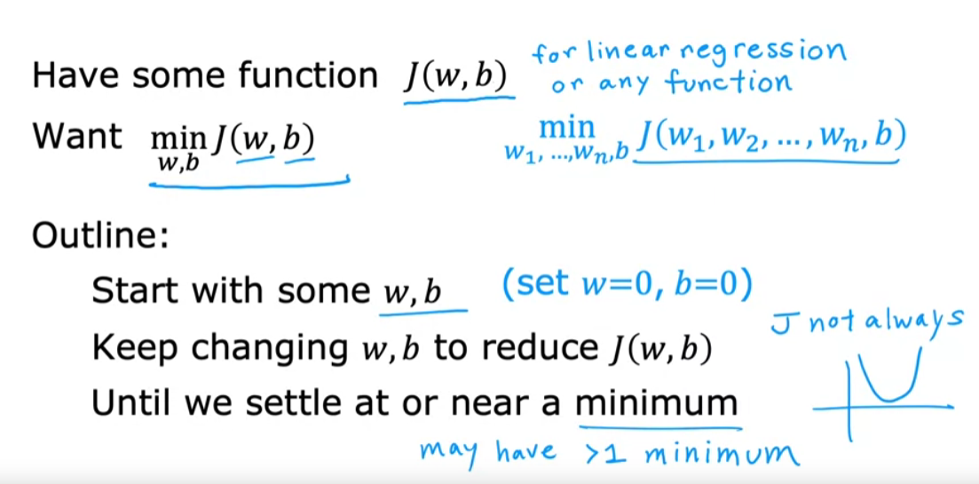
Gradient descent

It can be used for any optimization linear regresion as well as deep learning.

In the context of machine learning and optimization, “gradient” and “descent” in “gradient descent” refer to specific mathematical and conceptual elements used in the algorithm for finding the minimum of a function.

Gradient

The gradient is a vector that contains the partial derivatives of a function with respect to its input variables. In simpler terms, it points in the direction of the greatest rate of increase of the function. For a function $ f(x_1, x_2, \ldots, x_n) $, the gradient is given by:

$ \nabla f = \left( \frac{\partial f}{\partial x_1}, \frac{\partial f}{\partial x_2}, \ldots, \frac{\partial f}{\partial x_n} \right) $

In the context of a loss function in machine learning, the gradient provides information on how to adjust the model parameters to decrease the loss.

Descent

“Descent” refers to the iterative process of moving in the direction opposite to the gradient in order to minimize the function. This is because the gradient points in the direction of the steepest ascent, so moving in the opposite direction (i.e., the negative gradient) will lead to the steepest decrease. The basic update rule for gradient descent is:

$ \theta{new} = \theta{old} - \eta \nabla f(\theta_{old}) $

Here:

• $ \theta_{old} $ are the current parameters.
• $ \theta_{new} $ are the updated parameters.
• $ \eta $ is the learning rate, a hyperparameter that controls the size of the step taken in the direction of the negative gradient.
• $ \nabla f(\theta_{old}) $ is the gradient of the function evaluated at the current parameters.

Gradient Descent Algorithm

1. Initialize the parameters (weights) randomly.
2. Compute the gradient of the loss function with respect to the parameters.
3. Update the parameters by moving them in the direction opposite to the gradient.
4. Repeat steps 2 and 3 until convergence (i.e., until the parameters do not change significantly or a maximum number of iterations is reached).

Variants of Gradient Descent

1. Batch Gradient Descent: Uses the entire dataset to compute the gradient at each step.
2. Stochastic Gradient Descent (SGD): Uses one randomly chosen data point to compute the gradient at each step.
3. Mini-batch Gradient Descent: Uses a small random subset of the dataset to compute the gradient at each step.

Each variant has its own trade-offs in terms of speed, accuracy, and computational efficiency.

Certainly! Let’s dive deeper into the three main types of gradient descent algorithms: Batch Gradient Descent, Stochastic Gradient Descent (SGD), and Mini-batch Gradient Descent.

Batch Gradient Descent

Overview:

Batch Gradient Descent calculates the gradient of the cost function with respect to the parameters for the entire dataset. This means that each update of the parameters is based on the entire dataset.

Process:

1. Compute Gradient: Calculate the gradient of the cost function with respect to each parameter by considering all training examples.
2. Update Parameters: Update the parameters using the average gradient computed.

Formula:

$ \theta{new} = \theta{old} - \eta \cdot \frac{1}{m} \sum_{i=1}^m \nabla f(\theta, x_i, y_i) $

where:

• $ \theta $ are the model parameters.
• $ \eta $ is the learning rate.
• $ m $ is the number of training examples.
• $ (x_i, y_i) $ are the training examples.

Pros:

• Convergence is guaranteed to be stable and smooth, as it uses the entire dataset to make updates.
• Can find the global minimum for convex functions.

Cons:

• Computationally expensive for large datasets as it requires going through the entire dataset to perform a single update.
• Not suitable for online learning where data arrives continuously.

Stochastic Gradient Descent (SGD)

Overview:

SGD updates the model parameters for each training example one at a time. Instead of calculating the gradient using the entire dataset, it uses only one data point randomly chosen from the dataset.

Process:

1. Shuffle Data: Randomly shuffle the training data.
2. Iterate Over Data: For each training example, calculate the gradient and update the parameters immediately.

Formula:

$ \theta{new} = \theta{old} - \eta \cdot \nabla f(\theta, x_i, y_i) $

where $ (x_i, y_i) $ is a single training example.

Pros:

• Faster updates as it updates parameters more frequently.
• Can escape local minima more effectively due to the noisy updates.
• Suitable for online learning.

Cons:

• Updates can be noisy, leading to high variance in the parameter updates.
• May not converge as smoothly and can oscillate around the minimum.

Mini-batch Gradient Descent

Overview:

Mini-batch Gradient Descent is a compromise between Batch Gradient Descent and SGD. It splits the training data into small batches and updates the parameters based on each mini-batch.

Process:

1. Create Mini-batches: Divide the training dataset into small, random subsets (mini-batches).
2. Iterate Over Mini-batches: For each mini-batch, compute the gradient and update the parameters.

Formula:

$ \theta{new} = \theta{old} - \eta \cdot \frac{1}{n} \sum_{i=1}^n \nabla f(\theta, x_i, y_i) $

where $ n $ is the mini-batch size, and $ (x_i, y_i) $ are the training examples in the mini-batch.

Pros:

• Provides a balance between the stability of Batch Gradient Descent and the efficiency of SGD.
• More computationally efficient than Batch Gradient Descent.
• Reduces the variance of parameter updates compared to SGD.

Cons:

• Still requires tuning of the mini-batch size, which can affect the performance.
• May not converge as smoothly as Batch Gradient Descent for very noisy data.

Summary

• Batch Gradient Descent uses the entire dataset, which ensures stable convergence but is computationally expensive.
• Stochastic Gradient Descent (SGD) uses one random data point, allowing faster updates and better handling of online data but can be noisy and less stable.
• Mini-batch Gradient Descent uses small batches, offering a compromise with faster updates and reduced variance compared to SGD while being more efficient than Batch Gradient Descent.

In linear regression, \(f_{w,b}(x^{(i)}) = w*x^{(i)}+b\)

we utilize input training data to fit the parameters $w$,$b$ by minimizing a measure of the error between our predictions $f_{w,b}(x^{(i)})$ and the actual data $y^{(i)}$. The measure is called the $cost$, $J(w,b)$. In training we measure the cost over all of our training samples $x^{(i)},y^{(i)}$.

\[\text{Objective - } min (J_{w,b}) = \frac{1}{2m}\sum\limits_{i=1}^{m-1} (f_{w,b}(x^{(i)}) - y^{(i)})^2\]

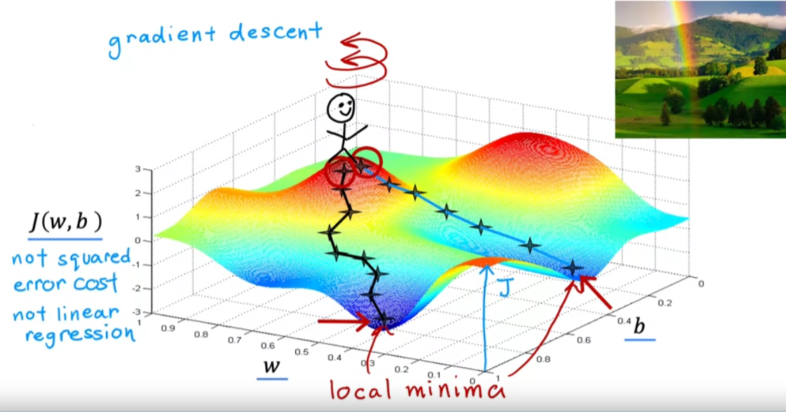
This cost function graph is for deep learning.For linear regression mostly it is in convex shape.

Simultaneously update w and b,

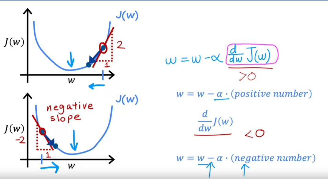
\[\text{repeat until converge } \begin{cases} w := w - \alpha \frac{\partial J(w,b)}{\partial w} \\ b := b - \alpha \frac{\partial J(w,b)}{\partial b} \end{cases}\]

After updating w, pre-updated w should be passed while calculating $\frac{\partial J(w,b)}{\partial b}$

if $\frac{\partial J(w,b)}{\partial w}$ is slope when +ve -> w decreases (moves towards left) -ve -> w increases (moves towards right)

the gradient descent is with gradient of cost w.r.t to w and b

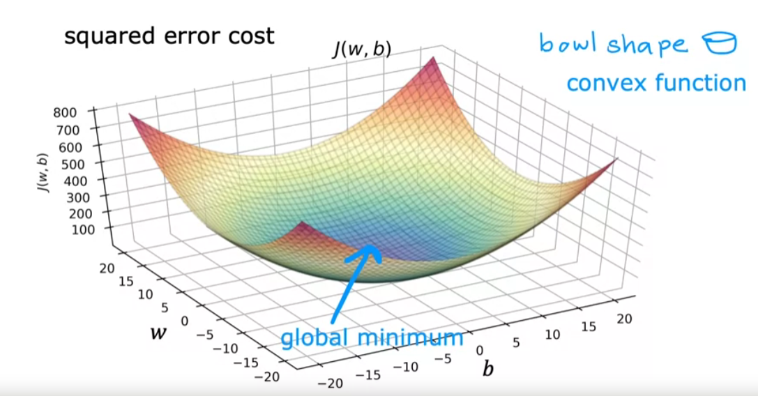
\[\text{repeat until converge } \begin{cases} w := w - \alpha \frac{1}{m}\sum\limits_{i=1}^{m-1} (f_{w,b}(x^{(i)}) - y^{(i)})x^{(i)} \\ b := b - \alpha \frac{1}{m}\sum\limits_{i=1}^{m-1} (f_{w,b}(x^{(i)}) - y^{(i)}) \end{cases}\]

When using square error cost function,the cost function does not and will never have multiple local minima. It has a single global minimum because of this bowl-shape. The technical term for this is that this cost function is a convex function. Informally, a convex function is of bowl-shaped function and it cannot have any local minima other than the single global minimum. When you implement gradient descent on a convex function, one nice property is that so long as you’re learning rate is chosen appropriately, it will always converge to the global minimum.

Here’s a plot of the model and data on the upper left and a contour plot of the cost function on the upper right and at the bottom is the surface plot of the same cost function. Often w and b will both be initialized to 0, but for this demonstration, lets initialized w = -0.1 and b = 900. So this corresponds to f(x) = -0.1x + 900.

The cost is decreasing at each update. So the parameters w and b are following this trajectory.

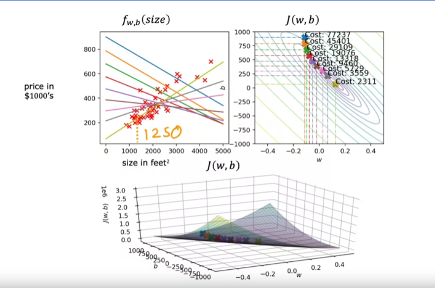
So in computing grading descent, when computing derivatives, batch gradient descent is computing the sum from i =1 to m, smaller subsets of the training data at each update step.

import numpy as np

def model_function(x,w,b):
    return np.dot(x,w)+b

def cost_function(x,y,w,b):
    m = x.shape[0]
    f_wb = model_function(x,w,b)
    total_loss =  (np.sum((f_wb - y)**2))/(2*m)
    return total_loss

def compute_gradient(x,y,w,b):
    m = x.shape[0]
    f_wb = model_function(x,w,b)
    dj_db = (1/m)*np.sum((f_wb - y))
    dj_dw = (1/m)*np.sum(x.T*(f_wb - y))
    return dj_dw,dj_db

def compute_gradient_descent(x,y,w,b,alpha,iterations=100):
    m = x.shape[0]

    for i in range(iterations):
        dj_dw,dj_db = compute_gradient(x,y,w,b)

        w = w - alpha *(1/m)* dj_dw
        b = b - alpha *(1/m)* dj_db

        if i%100==0:
            print(i,cost_function(x,y,w,b))
    return w,b

X_train = np.array([[2104, 5, 1, 45],
                    [1416, 3, 2, 40],
                    [852, 2, 1, 35]])
y_train = np.array([460, 232, 178])

w = np.random.rand(X_train.shape[1])
# w_init = np.array([ 0.39133535, 18.75376741, -53.36032453, -26.42131618])

# w = np.zeros_like(w_init)
b = 0
alpha = 5.0e-7
# dj_db,dj_dw = compute_gradient(x_train,y_train,w,b)
w_n ,b_n = compute_gradient_descent(X_train,y_train,w,b,alpha,1000)
print(w_n ,b_n)
for i in range(X_train.shape[0]):
    print(f"prediction: {np.dot(X_train[i], w_n) + b_n:0.2f}, target value: {y_train[i]}")

Result:

0 209314.1336159363
100 671.6664448665141
200 671.6661571235436
300 671.6658693815885
400 671.6655816406517
500 671.6652939007305
600 671.6650061618273
700 671.6647184239407
800 671.6644306870704
900 671.6641429512182
[ 0.2083132  -0.60111553 -0.18031452 -0.17953791] -0.0011102253224113373
prediction: 427.02, target value: 460
prediction: 285.62, target value: 232
prediction: 169.82, target value: 178

AdaGrad (Adaptive Gradient Algorithm)

AdaGrad is an optimization algorithm that adapts the learning rate for each parameter individually based on the historical gradients of each parameter. This allows it to perform well on problems with sparse gradients, such as natural language processing and certain computer vision tasks.

How AdaGrad Works:

1. Initialization:

   • Initialize parameters (weights) of the model.
   • Set the learning rate $\alpha$.
   • Initialize the accumulated squared gradients vector $G$ to zero.

2. Parameter Update:

   • For each parameter $\thetai$: $ G{t, i} = G{t-1, i} + g{t, i}^2 $
   • Here, $g_{t, i}$ is the gradient of the loss function with respect to $\theta_i$ at time step $t$.
   • Update the parameter $\thetai$: $ \theta{t, i} = \theta{t-1, i} - \frac{\alpha}{\sqrt{G{t, i}} + \epsilon} g_{t, i} $
   • $\epsilon$ is a small constant to prevent division by zero.

Key Features of AdaGrad:

• Adaptive Learning Rate: Each parameter has its own learning rate, which decreases over time, making AdaGrad particularly effective for dealing with sparse data.
• Learning Rate Decay: The learning rate for each parameter decreases over time due to the accumulation of past squared gradients, which can lead to better convergence.

RMSProp (Root Mean Square Propagation)

RMSProp is an optimization algorithm designed to overcome the diminishing learning rate problem of AdaGrad by using a moving average of squared gradients to scale the learning rate. This allows RMSProp to perform well on non-stationary and noisy problems.

How RMSProp Works:

1. Initialization:

   • Initialize parameters (weights) of the model.
   • Set the learning rate $\alpha$.
   • Initialize the moving average of squared gradients $E[g^2]$ to zero.
   • Set the decay rate $\beta$ (typically around 0.9).

2. Parameter Update:

   • For each parameter $\thetai$: $ E[g^2]{t, i} = \beta E[g^2]{t-1, i} + (1 - \beta) g{t, i}^2 $
   • Here, $g_{t, i}$ is the gradient of the loss function with respect to $\theta_i$ at time step $t$.
   • Update the parameter $\thetai$: $ \theta{t, i} = \theta{t-1, i} - \frac{\alpha}{\sqrt{E[g^2]{t, i}} + \epsilon} g_{t, i} $
   • $\epsilon$ is a small constant to prevent division by zero.

Key Features of RMSProp:

• Adaptive Learning Rate: The algorithm adapts the learning rate for each parameter based on a moving average of the squared gradients.
• Stability: By using a moving average, RMSProp can handle non-stationary and noisy problems more effectively than AdaGrad.
• Avoids Learning Rate Decay: Unlike AdaGrad, RMSProp does not let the learning rate decay too quickly, maintaining a more consistent learning rate throughout training.

Comparison:

• AdaGrad:

  • Pros: Effective for sparse data and features, handles infrequent features well.
  • Cons: Learning rate decreases continuously, which can lead to premature convergence.

• RMSProp:

  • Pros: Maintains a more consistent learning rate, effective for non-stationary and noisy problems.
  • Cons: Requires tuning of the decay rate hyperparameter.

Both algorithms are widely used in training machine learning models, and their choice depends on the specific characteristics of the problem at hand. RMSProp is often preferred for deep learning tasks due to its ability to handle varying data distributions during training.

The Adam algorithm,

short for Adaptive Moment Estimation, is an optimization algorithm used in training machine learning models, especially deep learning models. It combines the advantages of two other popular optimization algorithms: AdaGrad and RMSProp.

Here’s a breakdown of how the Adam algorithm works:

1. Initialization:

   • Initialize parameters (weights) of the model.
   • Initialize the first moment vector $ m_t $ and the second moment vector $ v_t $ to zero.
   • Set the learning rate $\alpha$, and hyperparameters $\beta_1$ (typically 0.9), $\beta_2$ (typically 0.999), and $\epsilon$ (a small constant to prevent division by zero, typically $10^{-8}$).

2. First Moment Estimate (Mean):

   • Compute the exponential moving average of the gradient (first moment) $ mt $: $ m_t = \beta_1 m{t-1} + (1 - \beta_1) g_t $
   • Here, $ g_t $ is the gradient at time step $ t $.

3. Second Moment Estimate (Variance):

   • Compute the exponential moving average of the squared gradient (second moment) $ vt $: $ v_t = \beta_2 v{t-1} + (1 - \beta_2) g_t^2 $

4. Bias Correction:

   • To counteract the bias introduced during the initial stages of training, compute bias-corrected estimates: $ \hat{m}_t = \frac{m_t}{1 - \beta_1^t} $ $ \hat{v}_t = \frac{v_t}{1 - \beta_2^t} $

5. Parameter Update:

   • Update the parameters (weights) using the following rule: $ \thetat = \theta{t-1} - \alpha \frac{\hat{m}_t}{\sqrt{\hat{v}_t} + \epsilon} $

Key Features of Adam:

• Adaptive Learning Rate: The algorithm adjusts the learning rate for each parameter individually, which can lead to faster convergence.
• Momentum: By maintaining a running average of past gradients, Adam helps to smooth out the optimization path, which can help in avoiding local minima and improving convergence.
• Combines Benefits of AdaGrad and RMSProp: Adam inherits the advantages of both AdaGrad (adaptation of learning rate based on past gradients) and RMSProp (scaling the learning rate using a moving average of squared gradients).

Advantages:

• Efficient: Requires little memory and is computationally efficient.
• Well-suited for Large Data: Works well with large datasets and high-dimensional parameter spaces.
• Default Choice: Often the default choice for many deep learning applications due to its robust performance.

Usage:

Adam is widely used in training neural networks, including convolutional neural networks (CNNs), recurrent neural networks (RNNs), and transformers. It is implemented in most deep learning frameworks such as TensorFlow, PyTorch, and Keras.

Stochastic Gradient Descent (SGD)

Stochastic Gradient Descent (SGD) is an optimization algorithm used to minimize the loss function in machine learning and deep learning models. It is a variant of the traditional Gradient Descent algorithm but differs in how it computes the gradient and updates the model parameters.

How SGD Works:

1. Initialization:

   • Initialize parameters (weights) of the model.
   • Set the learning rate $\alpha$.

2. Parameter Update:

   • Instead of using the entire dataset to compute the gradient, SGD uses a single data point (or a small batch) randomly chosen from the training dataset. This leads to faster updates and can escape local minima better than full-batch Gradient Descent.
   • For each training example $xi$ and its corresponding label $y_i$: $ \theta = \theta - \alpha \nabla\theta L(\theta; x_i, y_i) $
   • Here, $\theta$ represents the parameters, $\nabla_\theta L(\theta; x_i, y_i)$ is the gradient of the loss function $L$ with respect to $\theta$ evaluated at the single data point $(x_i, y_i)$, and $\alpha$ is the learning rate.

3. Iteration:

   • Repeat the parameter update for a specified number of iterations or until convergence.

Key Features of SGD:

• Stochastic Updates: By updating parameters using only a single or a small batch of training examples, SGD introduces noise into the optimization process. This noise can help the algorithm escape local minima and find a global minimum.
• Faster Convergence: SGD can converge faster than full-batch Gradient Descent, especially for large datasets, because it updates parameters more frequently.
• Scalability: SGD is more scalable to large datasets as it processes one example at a time, reducing memory requirements.

Advantages of SGD:

• Efficiency: Because it uses only one or a few examples to compute the gradient, it requires less computation per iteration compared to full-batch Gradient Descent.
• Regularization Effect: The noise introduced by stochastic updates can act as a form of regularization, potentially improving the generalization of the model.

Disadvantages of SGD:

• High Variance in Updates: The parameter updates in SGD can have high variance due to the noise introduced by using individual data points. This can lead to oscillations and slower convergence.
• Sensitivity to Learning Rate: The performance of SGD heavily depends on the choice of the learning rate. A learning rate that is too high can cause divergence, while a learning rate that is too low can result in slow convergence.

Variants of SGD:

To address some of the disadvantages of plain SGD, several variants have been developed:

1. Mini-batch SGD: Instead of using a single data point, mini-batch SGD uses a small batch of data points to compute the gradient, reducing the variance in updates while still being more efficient than full-batch Gradient Descent.
2. SGD with Momentum: Introduces a momentum term to smooth out the updates and accelerate convergence by accumulating a velocity vector in the direction of persistent reduction in the loss function.
3. SGD with Learning Rate Schedules: Adjusts the learning rate during training, such as decreasing the learning rate over time, to improve convergence.

Usage:

SGD and its variants are widely used in training various machine learning models, including linear regression, logistic regression, and deep neural networks. It is implemented in most machine learning and deep learning frameworks such as TensorFlow, PyTorch, and Keras.

In summary, SGD is a fundamental optimization technique in machine learning and deep learning that offers efficiency and scalability, making it suitable for large-scale problems. Its stochastic nature introduces both challenges and opportunities, which can be managed using various enhancements and techniques.

Loss Function

These loss functions are fundamental components in building and training neural networks, providing a way to quantify how well the model is performing and guide the optimization process during training.

1. nn.L1Loss

Description:

• Measures the Mean Absolute Error (MAE) between each element in the input $ x $ and target $ y $.
• Also known as the L1 Loss or L1 Norm Loss.

Formula: $ \text{L1Loss}(x, y) = \frac{1}{n} \sum_{i=1}^{n} |x_i - y_i| $

Usage:

• Suitable for regression problems where the error magnitude is more important than the squared error.

2. nn.MSELoss

Description:

• Measures the Mean Squared Error (MSE) between each element in the input $ x $ and target $ y $.
• Also known as the L2 Loss or L2 Norm Loss.

Formula: $ \text{MSELoss}(x, y) = \frac{1}{n} \sum_{i=1}^{n} (x_i - y_i)^2 $

Usage:

• Commonly used in regression problems where larger errors are significantly more undesirable than smaller ones.

3. nn.CrossEntropyLoss

Description:

• Computes the Cross Entropy Loss between input logits and target.
• Combines nn.LogSoftmax and nn.NLLLoss in one single class.

Formula: $ \text{CrossEntropyLoss}(x, y) = - \sum{i=1}^{n} y_i \log\left(\frac{e^{x_i}}{\sum{j=1}^{n} e^{x_j}}\right) $

Usage:

• Widely used in classification problems, especially when dealing with multi-class classification.

4. nn.CTCLoss

Description:

• The Connectionist Temporal Classification (CTC) loss.
• Used for sequence-to-sequence problems where the alignment between input and target sequences is unknown.

Usage:

• Commonly used in speech recognition and handwriting recognition.

5. nn.NLLLoss

Description:

• The Negative Log Likelihood Loss.
• Often used in combination with nn.LogSoftmax.

Formula: $ \text{NLLLoss}(x, y) = - \frac{1}{n} \sum_{i=1}^{n} \log P(y_i | x_i) $

Usage:

• Suitable for classification problems.

6. nn.PoissonNLLLoss

Description:

• Negative Log Likelihood Loss with Poisson distribution of the target.

Formula: $ \text{PoissonNLLLoss}(x, y) = x - y \log(x) + \log(y!) $

Usage:

• Used when the target follows a Poisson distribution.

7. nn.GaussianNLLLoss

Description:

• Gaussian Negative Log Likelihood Loss.
• Measures the negative log likelihood of the target under a Gaussian distribution.

Usage:

• Used in regression tasks where the output follows a Gaussian distribution.

8. nn.KLDivLoss

Description:

• The Kullback-Leibler Divergence Loss.
• Measures how one probability distribution diverges from a second, expected probability distribution.

Formula: $ \text{KLDivLoss}(P, Q) = \sum_{i} P(i) \log\left(\frac{P(i)}{Q(i)}\right) $

Usage:

• Often used in variational autoencoders and other probabilistic models.

9. nn.BCELoss

Description:

• Measures the Binary Cross Entropy between the target and the input probabilities.

Formula: $ \text{BCELoss}(x, y) = - \frac{1}{n} \sum_{i=1}^{n} [y_i \log(x_i) + (1 - y_i) \log(1 - x_i)] $

Usage:

• Used for binary classification problems.

Multiple Linear Regression

Multiple regression refers to a statistical technique that extends simple linear regression to handle the relationship between a dependent variable and two or more independent variables.

Multivariate Regression: Multivariate regression is a more general term that encompasses regression models with multiple dependent variables. It allows for the simultaneous modeling of the relationships between multiple independent variables and multiple dependent variables.

Gradient descent for multiple regression

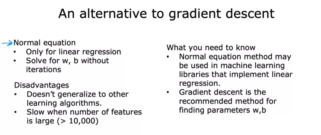
Normal Equation

The normal equation is a method used to find the optimal parameters (coefficients) for a linear regression model analytically. It provides a closed-form solution for the coefficients that minimize the cost function. Here is the normal equation for linear regression:

For a linear regression model with $n$ training examples, $m$ features, and a target variable, the normal equation is given by:

\[\theta = (X^TX)^{-1}X^TY\]

Where:

• $\theta$ is the vector of coefficients (parameters) that minimizes the cost function.
• $X$ is the matrix of features (design matrix) with dimensions $n \times (m+1)$, where each row represents a training example, and the first column is all ones (for the bias term).
• $Y$ is the vector of target values with dimensions $n \times 1$.

Steps to use the normal equation:

1. Feature Scaling: Ensure that the features are on a similar scale to help the optimization converge faster.

2. Add Bias Term: Include a column of ones in the feature matrix $X$ for the bias term.

3. Apply the Normal Equation: Use the formula to calculate the optimal coefficients $\theta$.

4. Make Predictions: Once you have the coefficients, you can use them to make predictions on new data.

It’s worth noting that while the normal equation provides an analytical solution, it may not be efficient for very large datasets because the matrix inversion operation $(X^TX)^{-1}$ has a time complexity of approximately $O(m^3)$, where $m$ is the number of features.

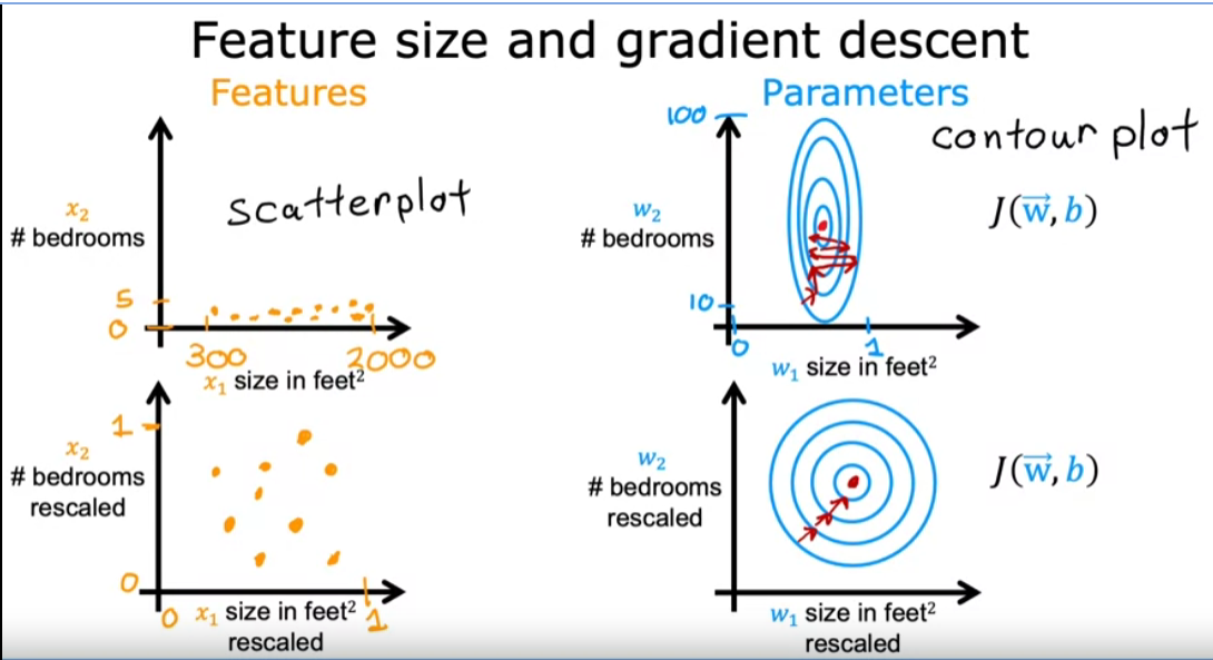
Feature Scaling

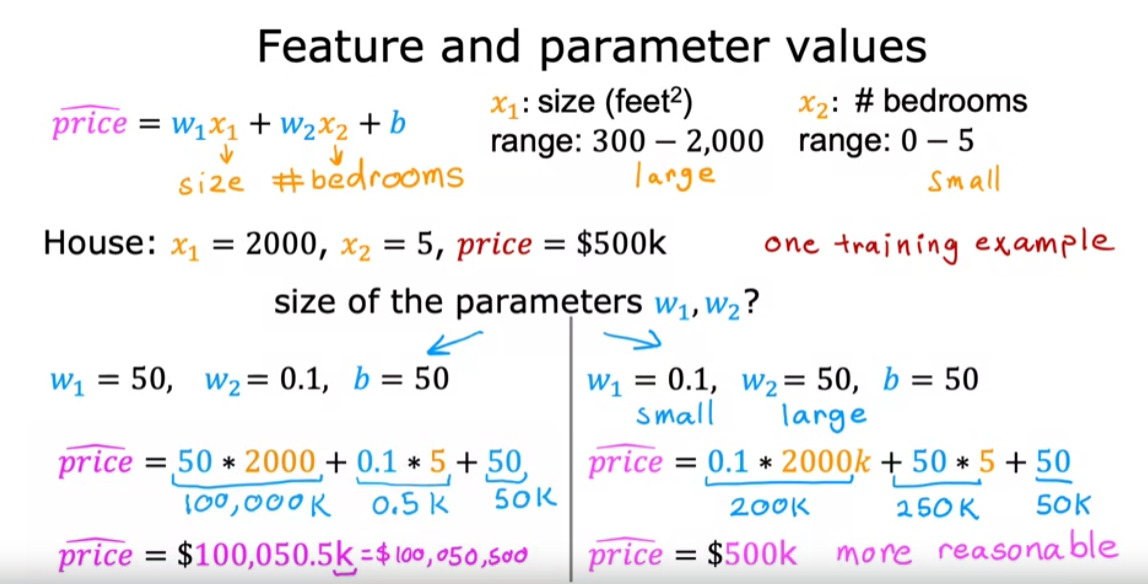
When a possible range of values of a feature is large, like the size and square feet which goes all the way up to 2000. It’s more likely that a good model will learn to choose a relatively small parameter value, like 0.1. Likewise, when the possible values of the feature are small, like the number of bedrooms, then a reasonable value for its parameters will be relatively large like 50.

A contour plot where the horizontal axis has a much narrower range, say between zero and one, whereas the vertical axis takes on much larger values, say between 10 and 100. So the contours form ovals or ellipses and they’re short on one side and longer on the other. And this is because a very small change to w1 can have a very large impact on the estimated price and that’s a very large impact on the cost J. Because w1 tends to be multiplied by a very large number, the size and square feet. In contrast, it takes a much larger change in w2 in order to change the predictions much. And thus small changes to w2, don’t change the cost function nearly as much.

Because the contours are so tall and skinny gradient descent may end up bouncing back and forth for a long time before it can finally find its way to the global minimum. In situations like this, a useful thing to do is to scale the features.

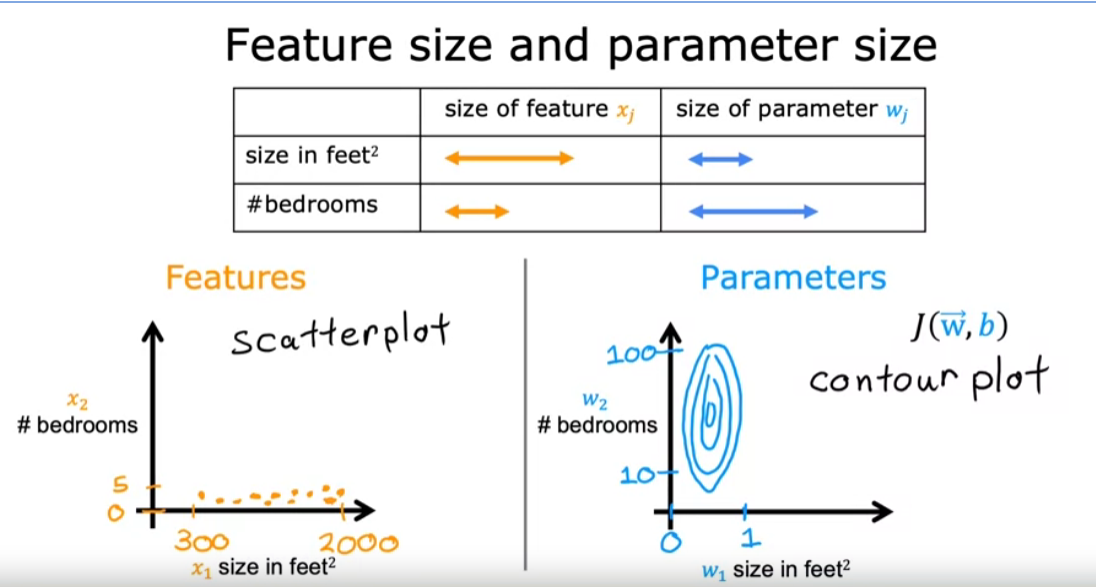
The key point is that the re scale x1 and x2 are both now taking comparable ranges of values to each other. And if you run gradient descent on a cost function to find on this, re scaled x1 and x2 using this transformed data, then the contours will look more like this more like circles and less tall and skinny. And gradient descent can find a much more direct path to the global minimum.

Feature Scaling

Feature scaling is a method used to normalize the range of independent variables or features of data. In data processing, it is also known as data normalization and is generally performed during the data preprocessing step.

min-max scaling

\[x_{norm} = \frac{x - x_{min}}{x_{max} - x_{min}}\]

standardization(standard scores (also called z scores))

\[x_{std} = \frac{x - \mu}{\sigma}\]

where $\mu$ is the mean (average) and $\sigma$ is the standard deviation from the mean

Polynomial Regression

When data doesn’t fit linearly,so try for higher dimensions.

Evaluate model

Mean Squared Error (MSE)

\(MSE = \frac{1}{n}\sum_{i=1}^{n}(y_i - \hat{y_i})^2\) \(or\) \(MSE = \frac{1}{2n}\sum_{i=1}^{n}(y_i - f(x_i))^2\) where

• $y_i$ is the true value and $\hat{y_i}$ is the predicted value
• $n$ is the number of observations

Root Mean Squared Error (RMSE)

\[RMSE = \sqrt{\frac{1}{n}\sum_{i=1}^{n}(y_i - \hat{y_i})^2}\]

R-squared (Coefficient of Determination)

\(R^2 = 1 - \frac{SS_{res}}{SS_{tot}}\) \(SS*{res} = \sum*{i=1}^{n}(y*i - \hat{y_i})^2\) \(SS*{tot} = \sum\_{i=1}^{n}(y_i - \bar{y_i})^2\)

where

• $SS_{res}$ is the sum of squares of residuals
• $SS_{tot}$ is the total sum of squares
• $y_i$ is the true value
• $\bar{y_i}$ is the mean of $y_i$
• $\hat{y_i}$ is the predicted value
• $n$ is the number of observations