Machine Learning Notes

Posted Nov 6, 2023

By ainotes 42 min read

each algo optimization function there working and comparison

l1 l2 regularization

Supervised Learning

http://www.stat.yale.edu/Courses/1997-98/101/linreg.htm#:~:text=A%20linear%20regression%20line%20has,y%20when%20x%20%3D%200

Extrapolation

Attempting to use a regression equation to predict values outside of this range is often inappropriate.This is called Extrapolation

Whenever a linear regression model is fit to a group of data, the range of the data should be carefully observed. Attempting to use a regression equation to predict values outside of this range is often inappropriate, and may yield incredible answers. This practice is known as extrapolation. Consider, for example, a linear model which relates weight gain to age for young children. Applying such a model to adults, or even teenagers, would be absurd, since the relationship between age and weight gain is not consistent for all age groups.

Adding Polynomial Feature

Polynomial regression is a form of regression analysis in which the relationship between the independent variable $x$ and the dependent variable $y$ is modelled as an $n$th degree polynomial in $x$.Rising the degree of the polynomial, we can get a more complex model.And the model will be more flexible and can fit the data better.

\[y = b + w_1x + w_2x^2 + w_3x^3 + ... + w_dx^d\]

where

$y$ is the target
$b$ is the bias
$w_1$ is the weight of feature $x$

  
# Import necessary libraries
import time
import numpy as np
import matplotlib.pyplot as plt
from sklearn.preprocessing import PolynomialFeatures, StandardScaler
from sklearn.linear_model import LinearRegression
from sklearn.metrics import mean_squared_error

# Assuming you have already split your data into X_train, X_test, y_train, and y_test

# Initiate polynomial features
poly = PolynomialFeatures(2, include_bias=False)

# Transform the x data for proper fitting (for single variable type it returns,[1,x,x**2])
X_train_poly = poly.fit_transform(X_train[['X3 distance to the nearest MRT station']])
X_test_poly = poly.transform(X_test[['X3 distance to the nearest MRT station']])

# Create a scaler object
scaler = StandardScaler()

# Fit the scaler to the training data and transform
X_train_scaled = scaler.fit_transform(X_train_poly)
X_test_scaled = scaler.transform(X_test_poly)

# Create a linear regression model
model = LinearRegression()
start_time = time.time()

# Train the model
model.fit(X_train_scaled, y_train)

time_taken_with_scaling = "{:.6f}".format(time.time() - start_time)
print("--- %s seconds ---" % (time_taken_with_scaling))

# Make predictions
y_pred = model.predict(X_test_scaled)

# accuracy
print('Mean squared error: %.2f' % mean_squared_error(y_test, y_pred))

# Plot the predictions on a scatter plot
plt.scatter(X_test_scaled[:, 1], y_test, color='blue')  # Use X_test_scaled[:, 1] for the x-axis
plt.scatter(X_test_scaled[:, 1], y_pred, color='red')    # Use X_test_scaled[:, 1] for the x-axis
plt.xlabel('X3 distance to the nearest MRT station')
plt.ylabel('Y house price of unit area')
plt.show()

  
--- 0.001193 seconds ---
Mean squared error: 69.36

  
# Import necessary libraries
import numpy as np
import matplotlib.pyplot as plt
from sklearn.preprocessing import PolynomialFeatures, StandardScaler
from sklearn.linear_model import LinearRegression
from sklearn.metrics import mean_squared_error

# Initialize lists to store training and testing errors
training_errors = []
testing_errors = []
maxdegree = 10
# Loop through degrees 1 to 12 and store the training and testing errors
for degree in range(1, maxdegree):
    # Initiate polynomial features
    poly = PolynomialFeatures(degree, include_bias=False)

    # Transform the x data for proper fitting (for single variable type it returns,[1,x,x**2])
    X_train_poly = poly.fit_transform(X_train[['X3 distance to the nearest MRT station']])
    X_test_poly = poly.transform(X_test[['X3 distance to the nearest MRT station']])

    # Create a scaler object
    scaler = StandardScaler()

    # Fit the scaler to the training data and transform
    X_train_scaled = scaler.fit_transform(X_train_poly)
    X_test_scaled = scaler.transform(X_test_poly)

    # Create a linear regression model
    model = LinearRegression()

    # Train the model
    model.fit(X_train_scaled, y_train)

    # Make predictions on both training and testing sets
    y_train_pred = model.predict(X_train_scaled)
    y_test_pred = model.predict(X_test_scaled)

    # Calculate mean squared errors for both training and testing sets
    mse_train = mean_squared_error(y_train, y_train_pred)/2
    mse_test = mean_squared_error(y_test, y_test_pred)/2

    # Append errors to the lists
    training_errors.append(mse_train)
    testing_errors.append(mse_test)

# Plot the training and testing errors against degree
plt.plot(range(1, maxdegree), training_errors, color='blue', label='Training')
plt.plot(range(1, maxdegree), testing_errors, color='red', label='Testing')
plt.xlabel('Degree of Polynomial')
plt.ylabel('Mean Squared Error')
plt.legend()
plt.show()

degree = np.argmin(testing_errors) + 1
print(f"Lowest CV MSE is found in the model with degree= {degree} and training error= {training_errors[degree-1]} and testing error= {testing_errors[degree-1]}")

  
# same process to choose bet diff neural network models
import numpy as np
import matplotlib.pyplot as plt
from sklearn.preprocessing import PolynomialFeatures, StandardScaler
from sklearn.linear_model import LinearRegression
from sklearn.metrics import mean_squared_error
from tensorflow.keras.models import Sequential
from tensorflow.keras.layers import Dense
from tensorflow.keras.optimizers import Adam
import tensorflow as tf
def build_bc_models():

    tf.random.set_seed(20)

    model_1_bc = Sequential(
        [
            Dense(25, activation = 'relu'),
            Dense(15, activation = 'relu'),
            Dense(1, activation = 'sigmoid')
        ],
        name='model_1_bc'
    )

    model_2_bc = Sequential(
        [
            Dense(20, activation = 'relu'),
            Dense(12, activation = 'relu'),
            Dense(12, activation = 'relu'),
            Dense(20, activation = 'relu'),
            Dense(1, activation = 'sigmoid')
        ],
        name='model_2_bc'
    )

    model_3_bc = Sequential(
        [
            Dense(32, activation = 'relu'),
            Dense(16, activation = 'relu'),
            Dense(8, activation = 'relu'),
            Dense(4, activation = 'relu'),
            Dense(12, activation = 'relu'),
            Dense(1, activation = 'sigmoid')
        ],
        name='model_3_bc'
    )

    models_bc = [model_1_bc, model_2_bc, model_3_bc]

    return models_bc

models_bc = build_bc_models()

poly = PolynomialFeatures(degree=1, include_bias=False)

# Transform the x data for proper fitting (for single variable type it returns,[1,x,x**2])
X_train_poly = poly.fit_transform(X_train[['X3 distance to the nearest MRT station']])
X_test_poly = poly.transform(X_test[['X3 distance to the nearest MRT station']])

# Create a scaler object
scaler = StandardScaler()

# Fit the scaler to the training data and transform
X_train_scaled = scaler.fit_transform(X_train_poly)
X_test_scaled = scaler.transform(X_test_poly)
# Initialize lists to store training and testing errors
training_errors = []

testing_errors = []

# Loop through models and store the training and testing errors

for model in models_bc:
    # Compile the model
    model.compile(loss='binary_crossentropy', optimizer=Adam(lr=0.001), metrics=['accuracy'])

    # Train the model
    model.fit(X_train_scaled, y_train, epochs=100, verbose=0)

    # Make predictions on both training and testing sets
    y_train_pred = model.predict(X_train_scaled)
    y_test_pred = model.predict(X_test_scaled)

    # Calculate mean squared errors for both training and testing sets
    mse_train = mean_squared_error(y_train, y_train_pred)/2
    mse_test = mean_squared_error(y_test, y_test_pred)/2

    # Append errors to the lists
    training_errors.append(mse_train)
    testing_errors.append(mse_test)

# Plot the training and testing errors against degree
plt.plot(range(1, len(models_bc)+1), training_errors, color='blue', label='Training')
plt.plot(range(1, len(models_bc)+1), testing_errors, color='red', label='Testing')
plt.xlabel('Model Number')
plt.ylabel('Mean Squared Error')
plt.legend()
plt.show()

model_number = np.argmin(testing_errors) + 1
print(f"Lowest CV MSE is found in the model number= {model_number} and training error= {training_errors[model_number-1]} and testing error= {testing_errors[model_number-1]}")

Logistic Regression

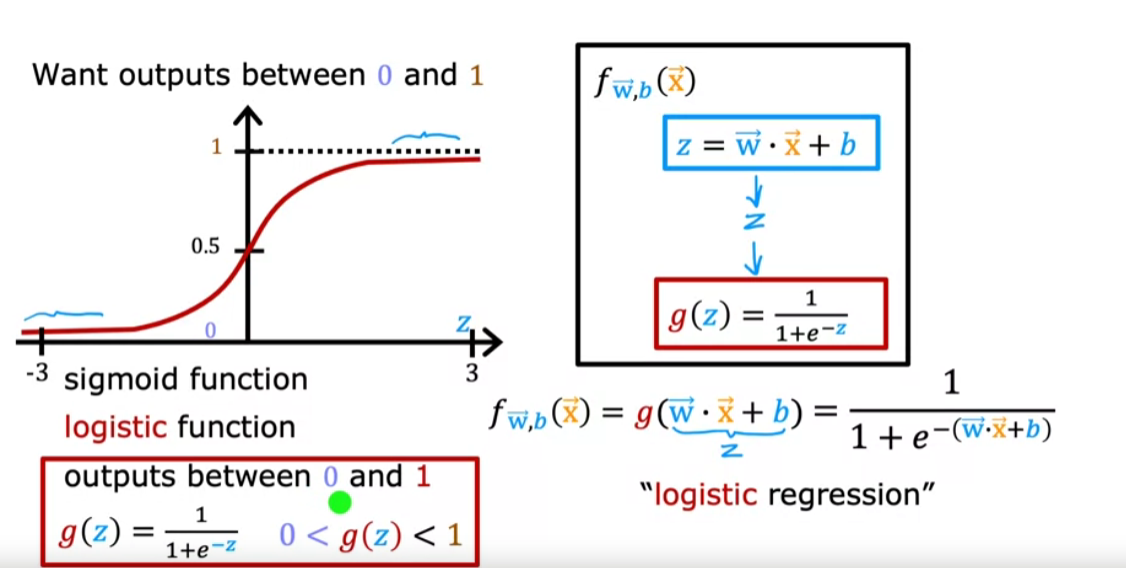
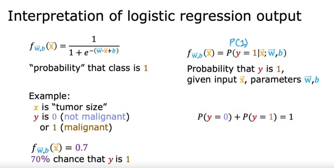
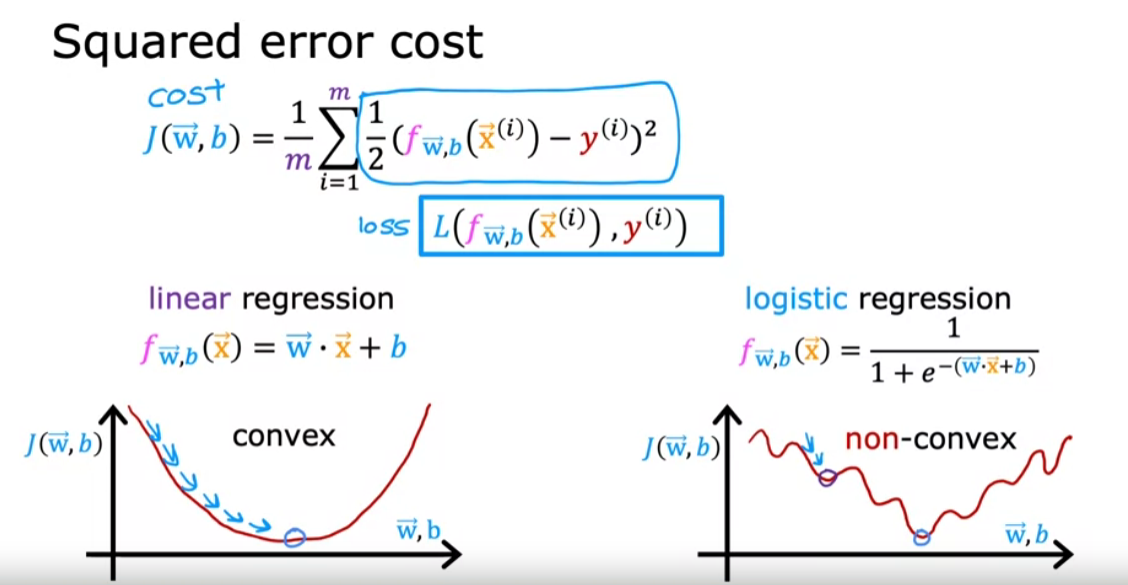
Logistic Regression uses a loss function more suited to the task of categorization where the target is 0 or 1 rather than any number.

Definition Note: In this course, these definitions are used:
Loss is a measure of the difference of a single example to its target value while the
Cost is a measure of the losses over the training set

This is defined:

$loss(f_{\mathbf{w},b}(\mathbf{x}^{(i)}), y^{(i)})$ is the cost for a single data point, which is:

\[\begin{equation} loss(f_{\mathbf{w},b}(\mathbf{x}^{(i)}), y^{(i)}) = \begin{cases}- \log\left(f_{\mathbf{w},b}\left( \mathbf{x}^{(i)} \right) \right) & \text{if $y^{(i)}=1$}\\- \log \left( 1 - f_{\mathbf{w},b}\left( \mathbf{x}^{(i)} \right) \right) & \text{if $y^{(i)}=0$} \end{cases} \end{equation}\]

$f_{\mathbf{w},b}(\mathbf{x}^{(i)})$ is the model’s prediction, while $y^{(i)}$ is the target value.
$f_{\mathbf{w},b}(\mathbf{x}^{(i)}) = g(\mathbf{w} \cdot\mathbf{x}^{(i)}+b)$ where function $g$ is the sigmoid function.

The defining feature of this loss function is the fact that it uses two separate curves. One for the case when the target is zero or ($y=0$) and another for when the target is one ($y=1$). Combined, these curves provide the behavior useful for a loss function, namely, being zero when the prediction matches the target and rapidly increasing in value as the prediction differs from the target. Consider the curves below:

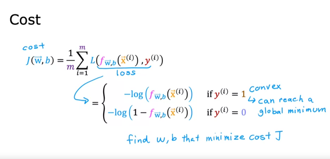
The loss function above can be rewritten to be easier to implement. $loss(f_{\mathbf{w},b}(\mathbf{x}^{(i)}), y^{(i)}) = (-y^{(i)} \log\left(f_{\mathbf{w},b}\left( \mathbf{x}^{(i)} \right) \right) - \left( 1 - y^{(i)}\right) \log \left( 1 - f_{\mathbf{w},b}\left( \mathbf{x}^{(i)} \right) \right)$

This is a rather formidable-looking equation. It is less daunting when you consider $y^{(i)}$ can have only two values, 0 and 1. One can then consider the equation in two pieces:
when $ y^{(i)} = 0$, the left-hand term is eliminated:

\[\begin{align} loss(f_{\mathbf{w},b}(\mathbf{x}^{(i)}), 0) &= (-(0) \log\left(f_{\mathbf{w},b}\left( \mathbf{x}^{(i)} \right) \right) - \left( 1 - 0\right) \log \left( 1 - f_{\mathbf{w},b}\left( \mathbf{x}^{(i)} \right) \right) \\ &= -\log \left( 1 - f_{\mathbf{w},b}\left( \mathbf{x}^{(i)} \right) \right) \end{align}\]

and when $ y^{(i)} = 1$, the right-hand term is eliminated:

\[\begin{align} loss(f_{\mathbf{w},b}(\mathbf{x}^{(i)}), 1) &= (-(1) \log\left(f_{\mathbf{w},b}\left( \mathbf{x}^{(i)} \right) \right) - \left( 1 - 1\right) \log \left( 1 - f_{\mathbf{w},b}\left( \mathbf{x}^{(i)} \right) \right)\\ &= -\log\left(f_{\mathbf{w},b}\left( \mathbf{x}^{(i)} \right) \right) \end{align}\]

ROC Curve

Evaluates binary classification by showing how the true positive rate and false positive rate change with different discrimination thresholds.

A Receiver Operating Characteristic (ROC) curve is a graphical representation of the performance of a binary classification model at various classification thresholds. It illustrates the trade-off between the true positive rate (sensitivity) and the false positive rate (1 - specificity) as the discrimination threshold is varied.

Here’s how the ROC curve works:

	Predicted Positive	Predicted Negative
Actual Positive	True Positive (TP)	False Negative (FN)
Actual Negative	False Positive (FP)	True Negative (TN)

Binary Classification:
- The ROC curve is commonly used for binary classification problems, where the goal is to distinguish between two classes (positive and negative).
True Positive Rate (Sensitivity):
- The true positive rate (TPR), also known as sensitivity or recall, is the proportion of actual positive instances correctly predicted by the model. $TPR = \frac{TP}{TP + FN}$
False Positive Rate (1 - Specificity):
- The false positive rate (FPR), also known as the complement of specificity, is the proportion of actual negative instances incorrectly predicted as positive by the model. $FPR = \frac{FP}{FP + TN}$
Threshold Variation:
- The ROC curve is created by varying the discrimination threshold of the classifier and plotting the TPR against the FPR at each threshold.
- As the threshold increases, the TPR usually decreases, and the FPR also decreases.
Random Classifier Line:
- The ROC curve of a random classifier (one that makes predictions irrespective of the input features) is represented by a diagonal line from the bottom left to the top right (the line y = x).
Ideal Classifier Point:
- The ideal classifier would have a TPR of 1 and an FPR of 0, resulting in a point at the top left corner of the ROC curve.
Area Under the ROC Curve (AUC-ROC):
- The AUC-ROC value provides a single scalar measure of the performance of a binary classification model. A perfect classifier has an AUC-ROC value of 1, while a random classifier has an AUC-ROC of 0.5.
- AUC-ROC measures the area under the ROC curve.
Choosing the Threshold:
- The choice of the threshold depends on the specific requirements of the classification task. A higher threshold may prioritize specificity, while a lower threshold may prioritize sensitivity.
Use in Model Evaluation:
- ROC curves are widely used to evaluate the performance of classifiers, especially in situations where the class distribution is imbalanced.

the ROC curve provides a visual representation of the performance of a binary classification model across different discrimination thresholds. It is a valuable tool for understanding the trade-off between true positive rate and false positive rate and for selecting an appropriate threshold based on the specific needs of the application.

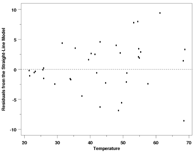
Residuals

Residual plots can help determine whether a model provides a good fit. Once a regression model has been fit to a group of data, examination of the residuals (the deviations from the fitted line to the observed values) allows the modeler to investigate the validity of his or her assumption that a linear relationship exists. Plotting the residuals on the y-axis against the explanatory variable on the x-axis reveals any possible non-linear relationship among the variables, or might alert the modeler to investigate lurking variables. In our example, the residual plot amplifies the presence of outliers.

A residual plot displays the residuals on the vertical axis and the independent variable on the horizontal axis. The ideal residual plot, called the null residual plot, shows a random scatter of points forming a band around the identity line.
A negative residual means that the predicted value is too high, and a positive residual means that the predicted value was too low.

evaluation metrics

Lurking Variables

A lurking variable is a third variable not considered in the model that significantly influences the relationship between two other variables.

If non-linear trends are visible in the relationship between an explanatory and dependent variable, there may be other influential variables to consider. A lurking variable exists when the relationship between two variables is significantly affected by the presence of a third variable which has not been included in the modeling effort. Since such a variable might be a factor of time (for example, the effect of political or economic cycles), a time series plot of the data is often a useful tool in identifying the presence of lurking variables.

Bias

Definition:
- Bias refers to the error introduced by approximating a real-world problem, which may be extremely complex, by a much simpler model.
- High bias implies that the model is too simplistic and unable to capture the underlying patterns in the data.
Characteristics:
- Models with high bias tend to oversimplify the relationships in the data and may perform poorly on both the training and unseen data.
- Commonly associated with underfitting.
Examples:
- A linear regression model applied to a dataset with a nonlinear underlying pattern may exhibit high bias.

Variance

Definition:
- Variance refers to the model’s sensitivity to small fluctuations or noise in the training data.
- High variance implies that the model is capturing not only the underlying patterns but also the noise in the data.
Characteristics:
- Models with high variance may perform well on the training data but poorly on unseen data, as they adapt too closely to the specific training dataset.
- Commonly associated with overfitting.
Examples:
- A complex polynomial regression model applied to a dataset with some random noise may exhibit high variance.

Bias-Variance Trade-Off

Trade-Off:
- There is often a trade-off between bias and variance. Increasing model complexity tends to decrease bias but increase variance, and vice versa.
- The goal is to find the right level of model complexity that minimizes both bias and variance, resulting in optimal predictive performance on new, unseen data.
Underfitting and Overfitting:
- Underfitting: Occurs when a model is too simple, leading to high bias and poor performance on both training and test data.
- Overfitting: Occurs when a model is too complex, capturing noise in the training data and leading to high variance. Performance on training data may be good, but it generalizes poorly to new data.
Model Evaluation:
- The bias-variance trade-off is crucial when evaluating models. Models should be assessed not only on their performance on training data but also on their ability to generalize to new, unseen data.
Regularization: Used to control the trade-off between bias and variance by penalizing overly complex models. Techniques such as regularization are used to control the trade-off between bias and variance by penalizing overly complex models.Helps prevent overfitting, making the model more generalizable to new, unseen data. Can improve the interpretability of the model by reducing the impact of irrelevant features.
- L1 Regularization (Lasso): Adds the absolute values of the coefficients as a penalty term to the objective function. It can lead to sparse models by encouraging some coefficients to become exactly zero.
- L2 Regularization (Ridge): Adds the squared values of the coefficients as a penalty term. It discourages overly large weights in the model.
- Elastic Net: Combines both L1 and L2 regularization. It is a linear combination of the L1 and L2 penalty terms.
Parameter Tuning: The strength of regularization is controlled by a hyperparameter (usually denoted as lambda or alpha). Higher values of this hyperparameter result in stronger regularization.
The appropriate value for the regularization hyperparameter is often determined through techniques like cross-validation.

Understanding the bias-variance trade-off is fundamental for selecting appropriate machine learning models, tuning hyperparameters, and achieving models that generalize well to new, unseen data.

Diagnose a model via Bias and Variance

Bias is the difference between the average prediction of our model and the correct value which we are trying to predict. A model with high bias pays very little attention to the training data and oversimplifies the model. It always leads to high error on training and test data.

Variance is the variability of model prediction for a given data point or a value which tells us spread of our data. A model with high variance pays a lot of attention to training data and does not generalize on the data which it hasn’t seen before. As a result, such models perform very well on training data but have high error rates on test data.

level of performance of a model:

human-level performance > training set performance > validation set performance > test set performance

High bias and low variance: model is underfitting
Low bias and high variance: model is overfitting
Low bias and low variance: model is good
High bias and high variance: model is bad

	High Variance	Low Variance
High Bias	Overfitting	Underfitting
Low Bias	bad	Good

Anomaly Detection Algorithms:

Here are all 20 Anomaly Detection Algorithms I could find and their Python Libraries:

📚 𝐒𝐜𝐢𝐤𝐢𝐭-𝐥𝐞𝐚𝐫𝐧

O͜͡ Density-based spatial clustering of applications with noise (DBSCAN) O͜͡ Isolation Forest O͜͡ Local Outlier Factor (LOF) O͜͡ One-Class Support Vector Machines (SVM) O͜͡ Principal Component Analysis (PCA) O͜͡ K-means O͜͡ Gaussian Mixture Model (GMM)

📚 𝐊𝐞𝐫𝐚𝐬/𝐓𝐞𝐧𝐬𝐨𝐫𝐅𝐥𝐨𝐰

O͜͡ Autoencoder

📚 𝐇𝐦𝐦𝐥𝐞𝐚𝐫𝐧

O͜͡ Hidden Markov Models (HMM)

📚 𝐏𝐲𝐎𝐃

O͜͡ Local Correlation Integral (LCI) O͜͡ Histogram-based Outlier Detection (HBOS) O͜͡ Angle-based Outlier Detection (ABOD) O͜͡ Clustering-Based Local Outlier Factor (CBLOF) O͜͡ Minimum Covariance Determinant (MCD) O͜͡ Stochastic Outlier Selection (SOS) O͜͡ Spectral Clustering for Anomaly Detection (SpectralResidual) O͜͡ Feature Bagging O͜͡ Average KNN O͜͡ Connectivity-based Outlier Factor (COF) O͜͡ Variational Autoencoder (VAE)

———————-

But how do we know which method is better?

🔖We don’t have labels in Unsupervised Learning, No ground Truth.

The answer lies in using evaluation metrics that can help us determine the quality of our algorithm.

———————-

🔬Evaluation Methods:

➊ Silhouette score:

A high Silhouette score (close to 1) indicates that data points within clusters are similar, and that the normal data points are well separated from the anomalous ones.

➋ Calinski-Harabasz index:

Calinski-Harabasz Index measures the between-cluster dispersion against within-cluster dispersion. A higher score signifies better-defined clusters.

➌ Davies-Bouldin index:

Davies-Bouldin Index measures the size of clusters against the average distance between clusters. A lower score signifies better-defined clusters.

➍ Kolmogorov-Smirnov statistic:

It measures the maximum difference between the cumulative distribution functions of the normal and anomalous data points.

➎ Precision at top-k:

The metric calculates the precision of the top-k anomalous data points using expert domain knowledge.

———————-

Dropout

Dropout is a regularization technique used to prevent overfitting in neural networks. It works by randomly “dropping out” (setting to zero) a fraction of the neurons during training. This forces the network to learn more robust features that are not dependent on specific neurons. Here’s why dropout is significant:

Prevents Overfitting: By randomly ignoring certain neurons during training, the network becomes less likely to rely on specific neurons and learns to generalize better.
Improves Generalization: It helps the network perform well on unseen data by making it more robust and less sensitive to the noise in the training data.
Acts as an Ensemble: At each training iteration, a different subset of the network is trained, which can be thought of as training an ensemble of smaller networks. During inference, all neurons are used, approximating the effect of averaging the predictions of many different networks.

Batch Normalization

Batch Normalization is a technique to improve the training of deep neural networks by normalizing the inputs of each layer so that they have a mean of zero and a standard deviation of one. Here’s why batch normalization is significant:

Stabilizes Learning: By normalizing the inputs, it mitigates the issue of internal covariate shift, where the distribution of inputs to a layer changes during training. This stabilization helps in faster convergence.
Allows Higher Learning Rates: It makes the training more stable, allowing the use of higher learning rates, which can speed up the training process.
Acts as Regularization: It has a slight regularization effect by adding noise to the training process, reducing the need for other regularization techniques like dropout.
Improves Gradient Flow: It reduces the problem of vanishing or exploding gradients, making it easier to train deeper networks.

In summary, dropout and batch normalization are two crucial techniques in modern deep learning. Dropout helps in preventing overfitting by randomly dropping neurons during training, while batch normalization stabilizes and accelerates training by normalizing the inputs of each layer. Both techniques contribute to building more efficient and effective neural networks.

Covariate shift is a situation in which the distribution of the model’s input features in production changes compared to what the model has seen during training and validation. Covariate shift is a change in the distribution of the model’s inputs between training and production data.

Bayes’ Theorem

Definition:

Bayes’ Theorem is a mathematical formula that describes the probability of an event based on prior knowledge of conditions that might be related to the event.
It is named after Thomas Bayes, an 18th-century statistician and theologian.

Formula: $ P(A|B) = \frac{P(B|A) \cdot P(A)}{P(B)} $

$ P(A B) $ is the probability of event A occurring given that B has occurred.
$ P(B A) $ is the probability of event B occurring given that A has occurred.
$ P(A) $ and $ P(B) $ are the probabilities of events A and B occurring independently.

Application:

Bayes’ Theorem is widely used in statistics, probability theory, and machine learning, especially in Bayesian statistics and Bayesian inference.

Naive Bayes

Definition:

Naive Bayes is a classification algorithm based on Bayes’ Theorem with the assumption that features are conditionally independent given the class label. This assumption simplifies the computation and leads to the term “naive.”

Types of Naive Bayes:

Gaussian Naive Bayes: Assumes that the features follow a Gaussian distribution.
Multinomial Naive Bayes: Commonly used for discrete data, such as text data (e.g., document classification).
Bernoulli Naive Bayes: Suitable for binary data (e.g., spam detection).

Assumption of Independence:

The “naive” assumption in Naive Bayes is that features are independent, which might not hold in real-world scenarios. Despite this simplification, Naive Bayes can perform well, especially in text classification tasks.

Application:

Naive Bayes is commonly used in spam filtering, text classification, sentiment analysis, and other tasks where the conditional independence assumption holds reasonably well.

Example: Text Classification with Naive Bayes

Suppose we want to classify an email as spam (S) or not spam (NS) based on the occurrence of words “free” and “discount.”

Features:

$ P(\text{“free”} S) = 0.8 $
$ P(\text{“discount”} S) = 0.6 $
$ P(\text{“free”} NS) = 0.1 $
$ P(\text{“discount”} NS) = 0.2 $

Prior Probabilities:

$ P(S) = 0.4 $
$ P(NS) = 0.6 $

Naive Bayes Calculation: $P(S|\text{"free", "discount"}) \propto P(S) \cdot P(\text{"free"}|S) \cdot P(\text{"discount"}|S)$ $P(NS|\text{"free", "discount"}) \propto P(NS) \cdot P(\text{"free"}|NS) \cdot P(\text{"discount"}|NS)$

By comparing the probabilities, we can classify the email as spam or not spam.

These concepts are foundational in probability theory, statistics, and machine learning, providing a basis for making probabilistic inferences and classifications.

Introduction to Navie Bayes

Navie Bayes is a classification algorithm based on Bayes’ theorem. According to Bayes’ theorem, the conditional probability of an event A, given another event B, is given by P(A

B) = P(B

A)P(A)/P(B). In the context of classification, we can think of P(A) as the prior probability of A, and P(A

B) as the posterior probability of A. In other words, we can think of the posterior probability as the probability of A given the data B.

Conditional Probability

Conditional probability is the probability of an event given that another event has occurred. For example, let’s say that we have two events A and B. The probability of A given that B has occurred is given by:

$P(A|B) = \frac{P(A \cap B)}{P(B)}$ where P(A ∩ B) is the probability of A and B occurring together.

Bayes’ Rule:

Probability of A given B is equal to the probability of interestion of A and B divided by the probability of B. $P(A|B) = \frac{P(A \cap B)}{P(B)}$ Similarly, we can write the probability of B given A as: $P(B|A) = \frac{P(A \cap B)}{P(A)}$

If we rearrange the above equation, we get: $P(A|B) = \frac{P(B|A)P(A)}{P(B)}$

In the context of classification, we can think of P(A) as the prior probability of A, and P(A

B) as the posterior probability of A. In other words, we can think of the posterior probability as the probability of A given the data B.

Navie Bayes Classifier

For tweets classification, we can use Navie Bayes classifier to classify tweets into positive and negative tweets.

\[\frac{P(\text{positive}|\text{tweet})}{P(\text{negative}|\text{tweet})} = \begin{cases} >1, & \text{positive} \\ <1, & \text{negative} \end{cases}\]

Laplacian Smoothing

We usually compute the probability of a word given a class as follows:

\[P(w_i|\text{class}) = \frac{\text{freq}(w_i, \text{class})}{N_{\text{class}}} \qquad \text{class} \in \{\text{Positive}, \text{Negative}\}\]

However, if a word does not appear in the training, then it automatically gets a probability of 0, to fix this we add smoothing as follows

\[P(w_i|\text{class}) = \frac{\text{freq}(w_i, \text{class}) + 1}{(N_{\text{class}} + V)}\]

Note that we added a 1 in the numerator, and since there are $V$ words to normalize, we add $V$ in the denominator.

$N_{\text{class}}$: number of words in class

$V$: number of unique words in vocabulary

Log Likelihood

We can use log likelihood to avoid underflow. The log likelihood is given by:

\[\lambda(w) = \log \frac{P(w|\text{pos})}{P(w|\text{neg})}\]

where $P(w

\text{pos})$ and $P(w

\text{neg})$ are computed using Laplacian smoothing.

train naïve Bayes classifier

Get or annotate a dataset with positive and negative tweets
Preprocess the tweets:
Lowercase, Remove punctuation, urls, names , Remove stop words , Stemming , Tokenize sentences
Compute $\text{freq}(w, \text{class})$:
Get $P(w \text{pos}), P(w \text{neg})$
Get $\lambda(w)$

\[\lambda(w) = \log \frac{P(w|\text{pos})}{P(w|\text{neg})}\]

Compute $\text{logprior}$

\[\text{logprior} = \log \frac{D_{\text{pos}}}{D_{\text{neg}}}\]

where $D_{\text{pos}}$ and $D_{\text{neg}}$ correspond to the number of positive and negative documents respectively.

Compute Score $\text{logprior} + \sum_{w \in \text{tweet}} \lambda(w) = \begin{cases} >1, & \text{positive} \\ <1, & \text{negative} \end{cases}$

Bayes Theorem -

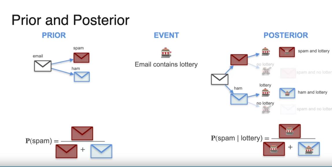
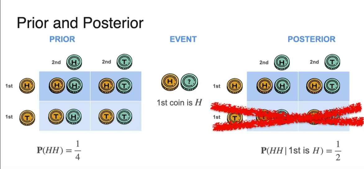
Prior and Posterior

Bayes’ theorem in action, where first you find the prior the probability that an email is spam, but just the initial probability, namely dividing the number of spam emails divided by the total number of emails. Then there was an event, for example, the email contains the word lottery and then a posterior which refined this probability by creating a tree of possibilities. This gave us four possibilities that the email was spam and lottery, that it was spam and no lottery, that it was ham and lottery, and that it was ham and no lottery. And then, you further calculated the probability of spam and lottery by forgetting all the emails that don’t contain the word lottery and doing the calculation there. Then the probability of spam given lottery is equal to the probability of spam and lottery divided by the sum of the probabilities of spam and lottery and ham and lottery and that was the posterior.

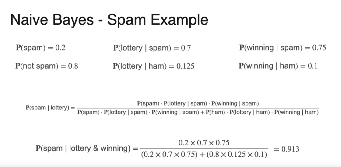
Naive Bayes

Naive Bayes is a probabilistic algorithm used for classification tasks, particularly in spam email filtering. The algorithm is based on Bayes’ theorem, which calculates the probability of an event based on prior knowledge of conditions related to that event. In the case of spam classification, Naive Bayes calculates the probability that an email is spam given the occurrence of certain words.

The challenge arises when dealing with multiple words (features). Calculating the joint probability of an email containing all these words can be problematic, especially if the dataset lacks instances where all words co-occur. The solution lies in the “naive” assumption that the appearances of words are independent, although this is not true in reality. Despite this simplification, Naive Bayes often produces effective results.

The algorithm calculates the posterior probability of an email being spam given certain words by multiplying the individual probabilities of each word given spam. This product is then normalized by adding similar products for the ham (non-spam) class. The result is a posterior probability that helps classify emails as spam or non-spam.

In a practical example, the Naive Bayes algorithm is applied to emails containing the words “lottery” and “winning.” The probabilities of these words given spam or ham are calculated, and the algorithm yields a posterior probability indicating the likelihood of an email being spam given the presence of these words. Naive Bayes is considered powerful and useful, especially when dealing with large feature sets in classification tasks.

Application of probablity in ML

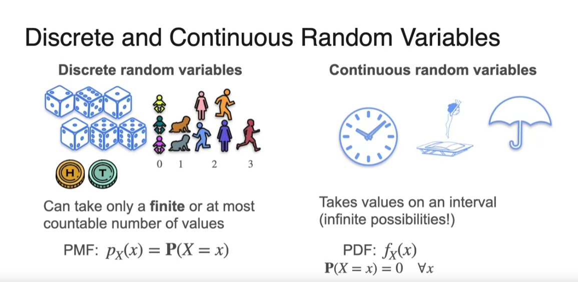
PMF

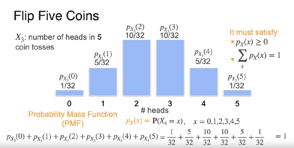
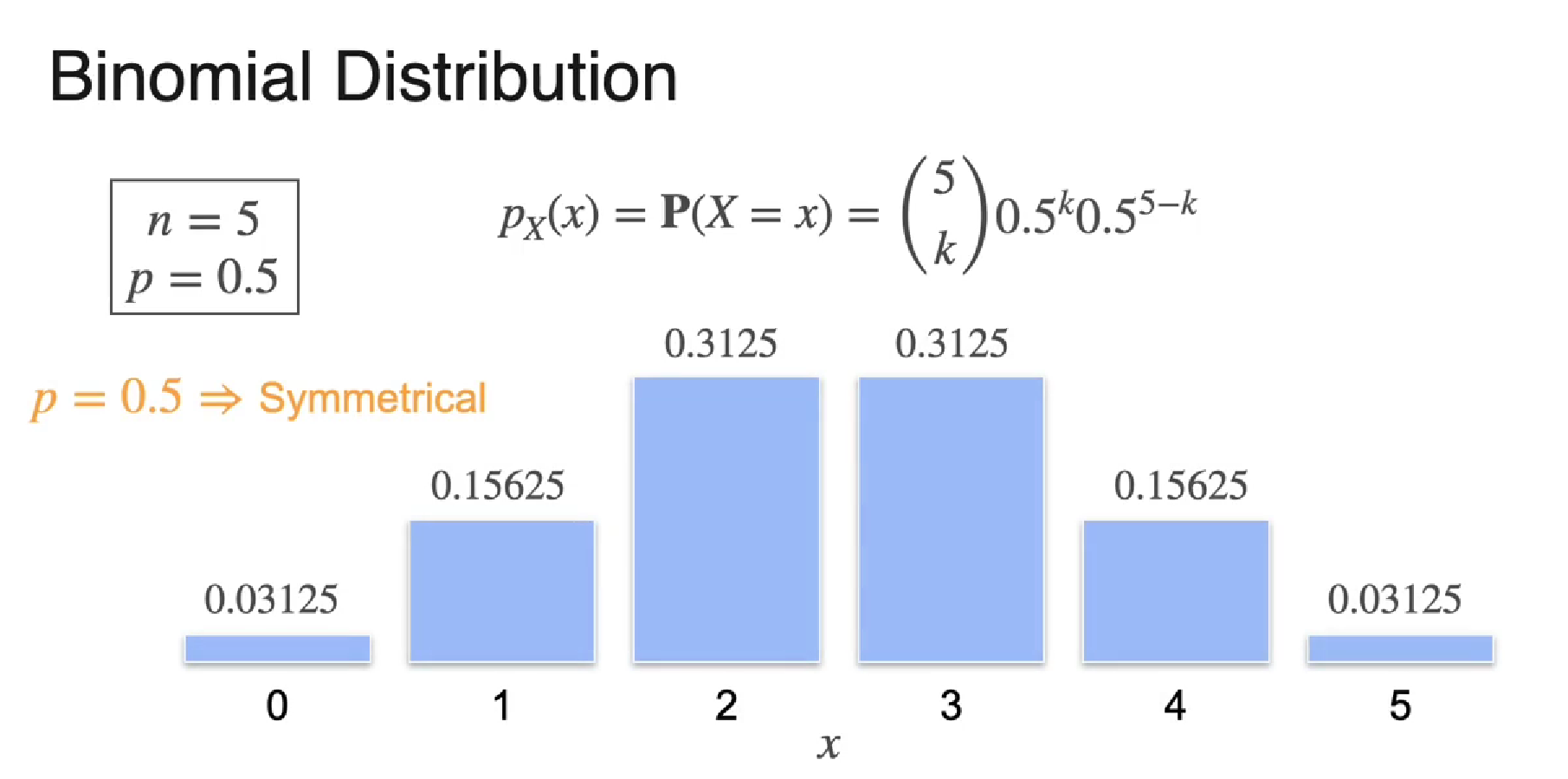
When p = 0.5

when p = 0.3 (biased coin)

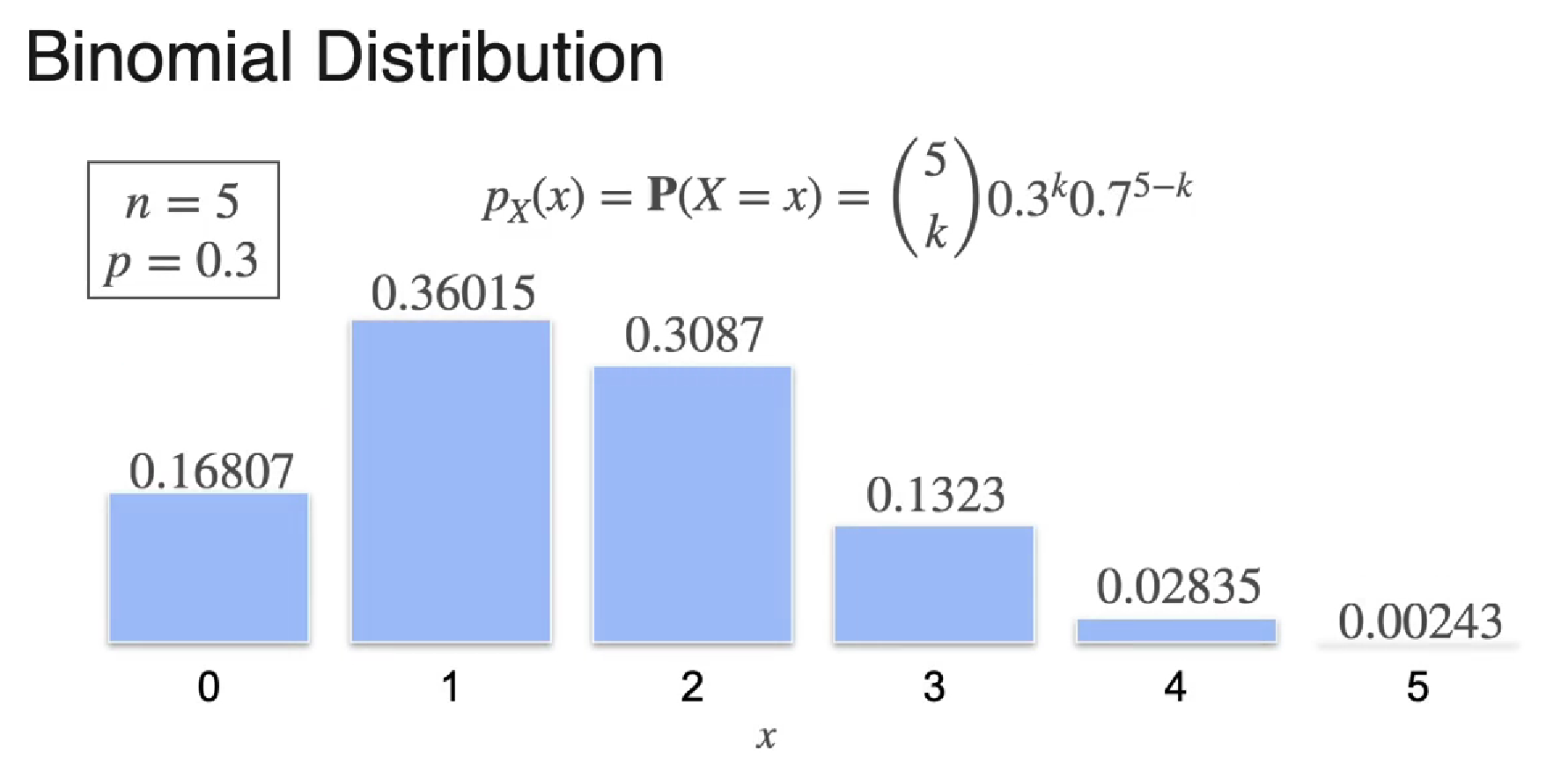
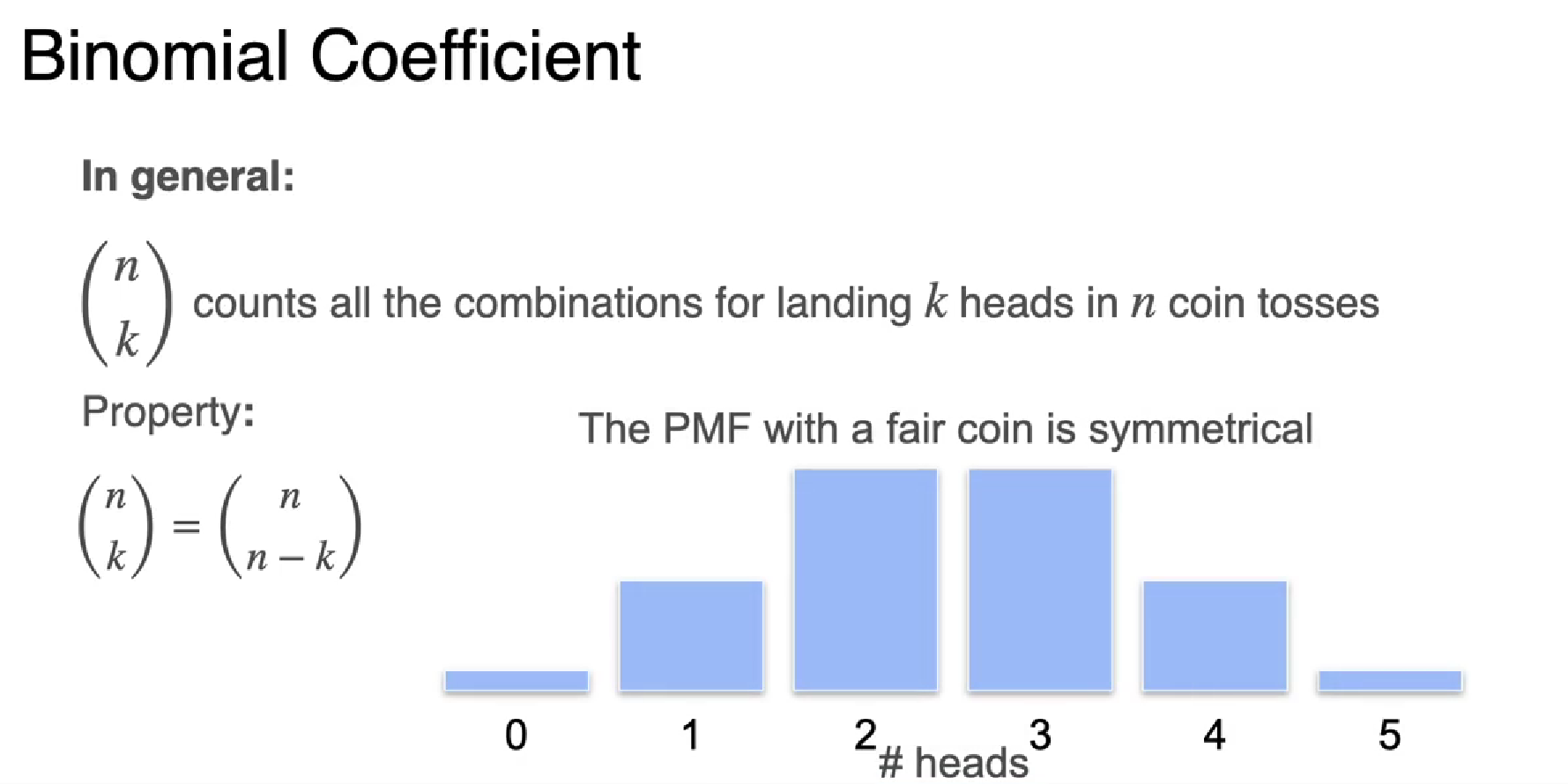
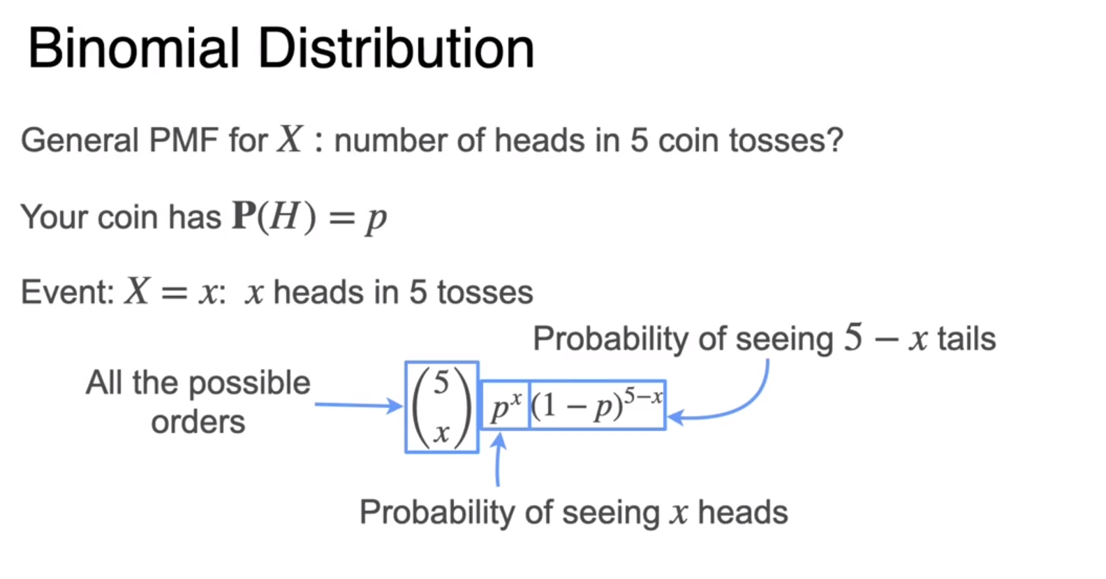
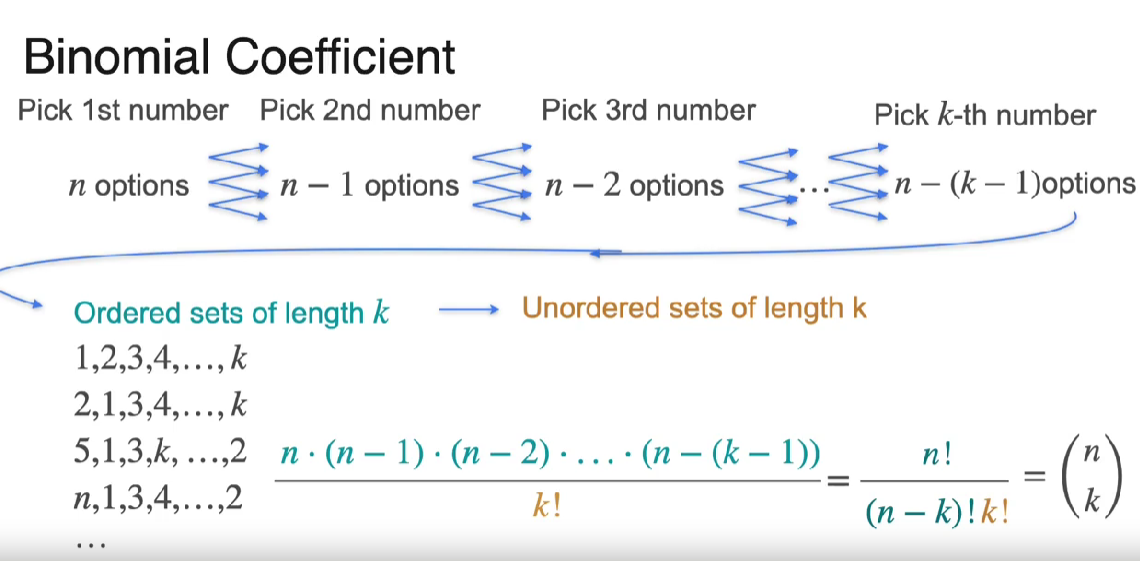
Derivation

Bernoulli distribution

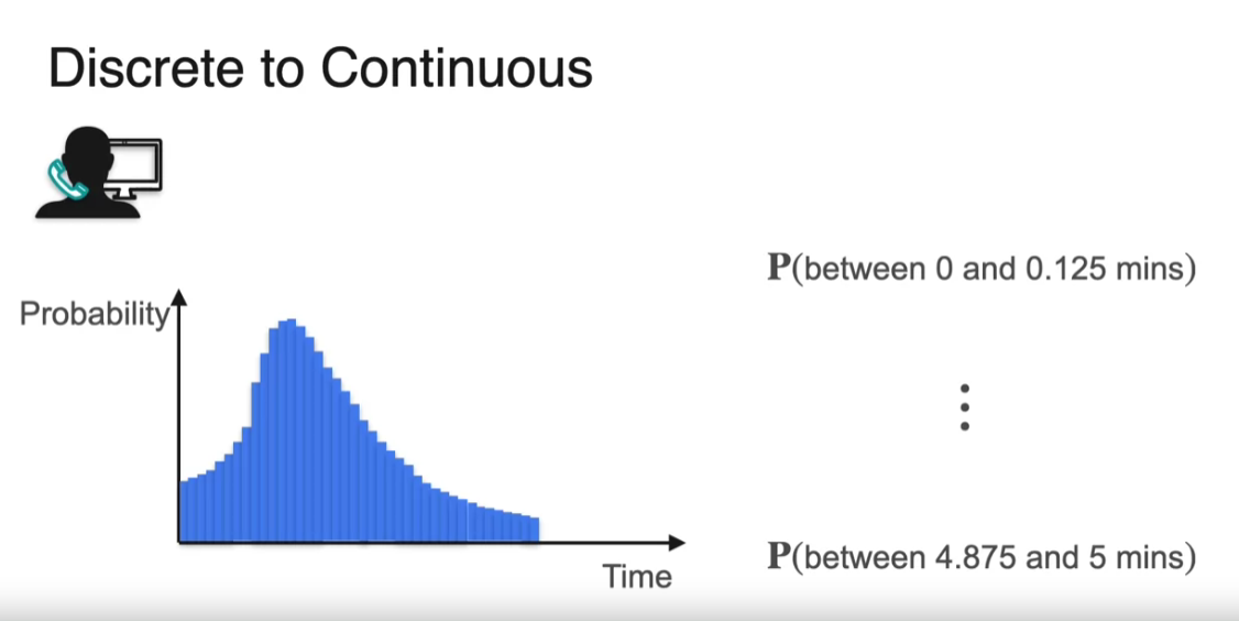
Continuous Distribution

We can continue splitting these intervals and getting discrete distributions. And if we were to do this infinitely many times, then what we get a continuous distribution. Imagine just a bunch of very, very skinny bars, infinitely many of them, that become just a curve. Now, in the discrete distribution, we had that the sum of heights have to be equal to 1. The sum of heights was the same as saying the blue area. So in the continuous distribution, we have the same condition, the area under the curve is equal to 1.

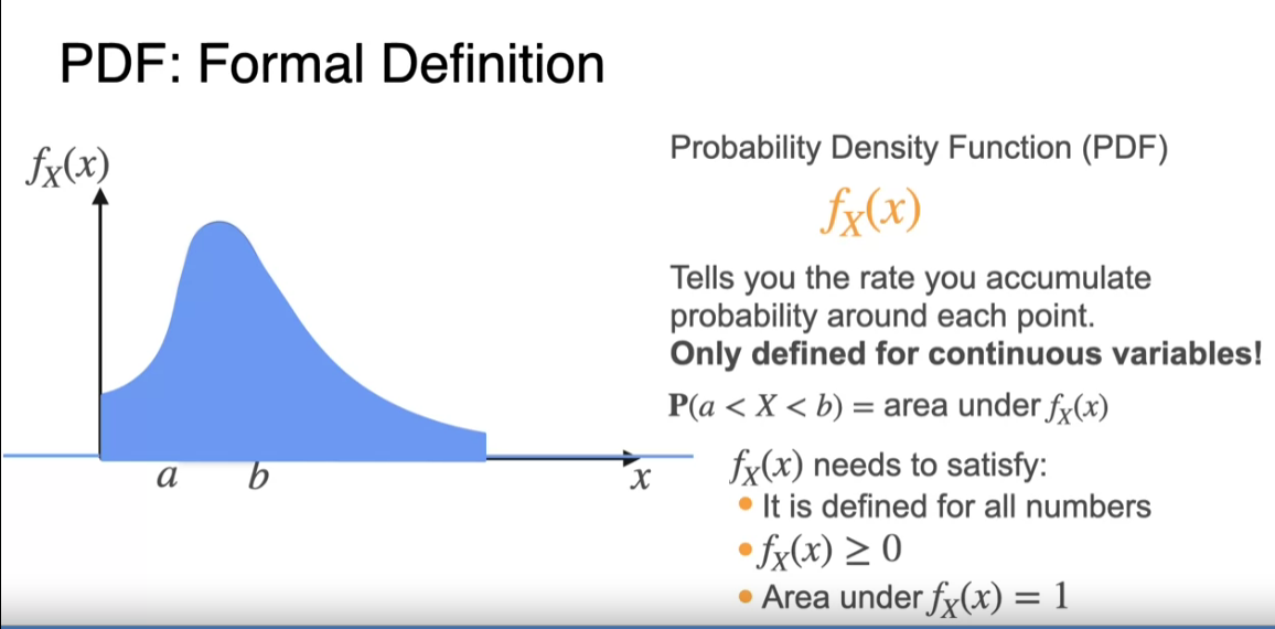
Probability Density Function

we divide the intervals into smaller and smaller, also the areas get smaller and smaller until they get to zero. So that’s why we have to look into intervals and not just heights. So as I told you before, this function is called a probability density function, or PDF for short, and it’s usually denoted as a lowercase f. It is the equivalent of the lowercase p in the discrete distribution. The equivalent of the mass function is now it’s called probability density function.

PDFs are a function defined only for continuous variables and it represents the rate at which you accumulate probability around each point. You can use the PDF to calculate probabilities. How do you do that? Simply by getting the area under the PDF curve between points A and B.

it needs to be defined for all the numbers in the real line. That means that it can actually be zero for many values. For example, before zero or after the cutoff at the right. But it doesn’t need to, it could be positive for all the numbers and the area still being 1 if it gets really, really, really tiny at the tails. And it also needs to be positive or 0 for all values.

And it also needs to be positive or 0 for all values. This is reasonable because otherwise it would get placed in negative probabilities.

the area under the curve has to be 1

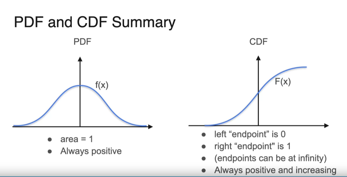
Summary PMF and PDF

Let’s take a look at discrete random variables, and remember, that they can only take a finite or at most accountable number of values. While continuous random variables are used to model experiments where the outcome can take any value in an interval. Because of this difference between discrete and continuous random variables, each kind will have their own way of describing the behavior and computing probabilities. To measure the probability of events in the case of a discrete random variable, you have a probability mass function, which is defined as the probability that x takes on a particular value. For the continuous random variable, you have the probability density function. And remember that for this type of variable, the probability that the variable takes on a particular value is always 0. So you need to look at areas on this side.

CDF

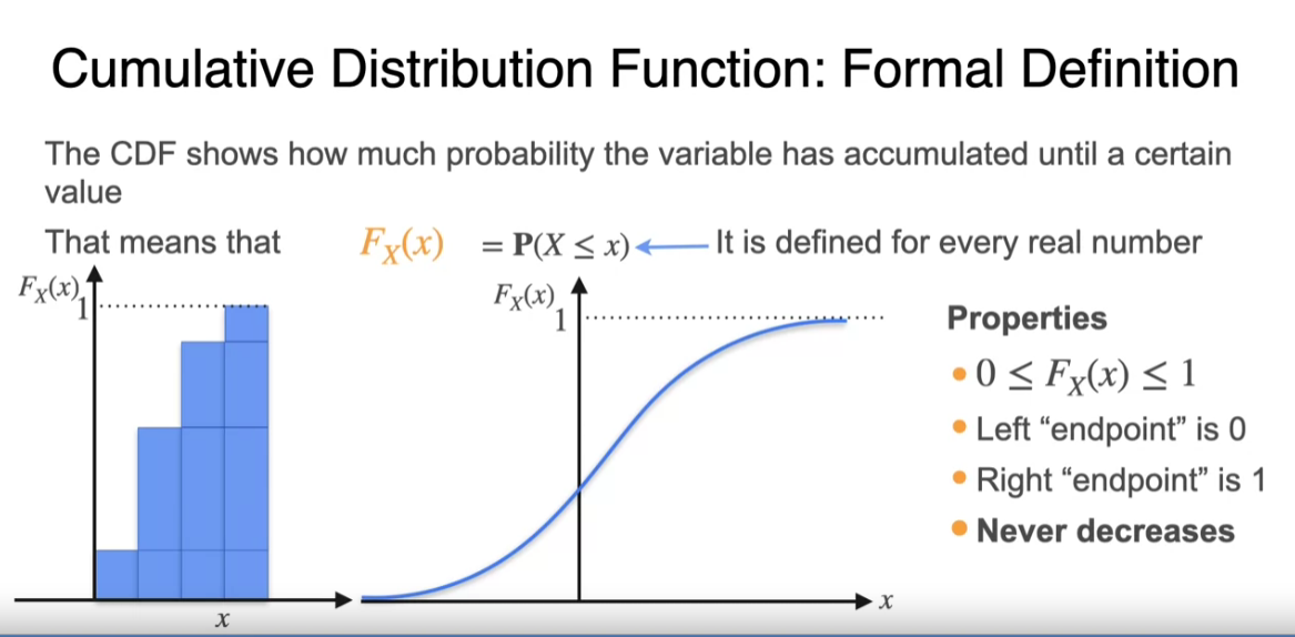
To really summarize, on the left, you have a PDF which is written as a function f(x), let’s say. It’s a function that’s always positive and has a total area of one underneath the curve. The CDF has a left endpoint of zero, our right endpoint of one, and it’s always positive, and it’s always increasing. Sometimes you’re going to be using the PDF, and some other times you’re going to be using the CDF depending on which one’s more convenient at the moment, but it’s good to know both really well.

These are evaluation metrics used to assess the performance of classification models, particularly in binary classification. Each metric has its own use case, and the choice of metric depends on the specific goals and context of your problem. Here’s an overview of each metric:

Accuracy (acc):
- Definition: The ratio of correctly predicted instances to the total instances.
- Use Case: Best used when the class distribution is balanced and all classes are equally important.
Balanced Accuracy:
- Definition: The average of recall obtained on each class.
- Use Case: Useful when the dataset is imbalanced.
MCC (Matthews Correlation Coefficient):
- Definition: Takes into account true and false positives and negatives and is generally regarded as a balanced measure.
- Use Case: Suitable for imbalanced datasets.
ROC AUC (roc_auc):
- Definition: The area under the Receiver Operating Characteristic curve.
- Use Case: Used for evaluating binary classifiers, particularly when classes are imbalanced.
ROC AUC OVO Macro (roc_auc_ovo_macro):
- Definition: Macro-averaged ROC AUC for one-vs-one classification.
- Use Case: Used for multiclass problems evaluated in a binary context.
Log Loss (log_loss, nll):
- Definition: Measures the performance of a classification model where the output is a probability value between 0 and 1.
- Use Case: Useful when you need probability outputs, and lower values indicate better performance.
PAC (Prediction Accuracy Classifier):
- Definition: Specific to the proportion of correct predictions.
- Use Case: Another form of accuracy.
PAC Score:
- Definition: Related to PAC, often used in specific contexts.
- Use Case: Similar to PAC.
Quadratic Kappa:
- Definition: A measure of inter-rater agreement or classifier performance that takes the agreement occurring by chance into account.
- Use Case: Useful in ordinal classification.
Average Precision:
- Definition: The average of the precision scores calculated at each threshold.
- Use Case: Evaluates the model’s ability to return relevant instances.
Precision:
- Definition: The ratio of true positive predictions to the total predicted positives.
- Use Case: Important when the cost of false positives is high.
Precision (macro, micro, weighted):
- Macro: Precision calculated independently for each class and then averaged.
- Micro: Precision calculated globally by counting total true positives and false positives.
- Weighted: Precision weighted by the number of true instances for each class.
- Use Case: Macro for class imbalances; micro and weighted for varying class sizes.
Recall:
- Definition: The ratio of true positive predictions to the total actual positives.
- Use Case: Important when the cost of false negatives is high.
Recall (macro, micro, weighted):
- Macro: Recall calculated independently for each class and then averaged.
- Micro: Recall calculated globally by counting total true positives and false negatives.
- Weighted: Recall weighted by the number of true instances for each class.
- Use Case: Macro for class imbalances; micro and weighted for varying class sizes.
F1 Score (f1):
- Definition: The harmonic mean of precision and recall.
- Use Case: Useful when you need a balance between precision and recall.
F1 Score (macro, micro, weighted):
- Macro: F1 score calculated independently for each class and then averaged.
- Micro: F1 score calculated globally by counting total true positives, false negatives, and false positives.
- Weighted: F1 score weighted by the number of true instances for each class.
- Use Case: Macro for class imbalances; micro and weighted for varying class sizes.

These metrics help you understand different aspects of model performance, and choosing the right one depends on the specific needs of your project and the nature of your data. For example, in highly imbalanced datasets, metrics like ROC AUC, F1 score, or MCC might be more informative than accuracy.

“binary”: [ “accuracy”, “acc”, “balanced_accuracy”, “mcc”, “roc_auc_ovo_macro”, “log_loss”, “nll”, “pac”, “pac_score”, “quadratic_kappa”, “roc_auc”, “average_precision”, “precision”, “precision_macro”, “precision_micro”, “precision_weighted”, “recall”, “recall_macro”, “recall_micro”, “recall_weighted”, “f1”, “f1_macro”, “f1_micro”, “f1_weighted” ]

The variance threshold is used to remove features with low variance, which are considered less informative for machine learning models. Here’s how it affects your model and its relationship with the target variable:

Impact on the Model: Reduction of Overfitting: Features with low variance may not contribute significant information to the model and can lead to overfitting. Removing these features helps in creating a more generalizable model. Model Complexity: Reducing the number of features decreases the complexity of the model, making it simpler and often improving its performance and interpretability. Training Time: Fewer features mean less data to process, which can reduce the training time for your model. Dependency on Target Variable: VarianceThreshold does not consider the target variable when selecting features; it purely looks at the variance of the features themselves. Therefore, features with low variance are not necessarily independent of the target variable, but they are less likely to be useful because they provide little variability for the model to learn from.

To assess the dependency of features on the target variable, you should use feature selection techniques that consider the relationship between features and the target variable, such as:

Correlation Coefficient: Calculate the correlation between each feature and the target variable. Features with high correlation (positive or negative) are more likely to be important. Mutual Information: Measures the mutual dependence between the feature and the target variable. Feature Importance from Tree-based Models: Tree-based models like Random Forests and Gradient Boosting provide feature importance scores. Univariate Feature Selection: Use statistical tests to select features based on their univariate statistical significance (e.g., SelectKBest with f_classif).

Significance of P-value: P-value Definition:

The p-value indicates the probability that the observed relationship between a feature and the target variable is due to chance. Lower p-values suggest stronger evidence against the null hypothesis (which states that there is no relationship between the feature and the target variable). Thresholds for Significance:

Common thresholds for significance are 0.05, 0.01, or 0.001. If a feature has a p-value less than the chosen threshold, it is considered statistically significant and likely has a meaningful relationship with the target variable. Feature Selection:

Features with low p-values (below the threshold) are typically considered important and are selected for use in the model. Features with high p-values are considered less important or irrelevant and can be removed.

Interpreting P-values in Your Context: In the context of your dataset and feature selection process, the p-values help you determine which features are likely to be informative for predicting the target variable ‘C’. Here’s a step-by-step explanation using your dataset:

Load and Preprocess Data:

Convert datetime columns to numerical format and standardize the features. Apply VarianceThreshold:

Remove features with low variance that are unlikely to be informative. Statistical Test (ANOVA F-test):

Use SelectKBest with the f_classif function to perform an ANOVA F-test between each feature and the target variable. Obtain p-values for each feature indicating their significance. Interpret P-values:

Low p-values (< 0.05, for example) suggest that the feature is significantly related to the target variable and should be considered in the model. High p-values (> 0.05) suggest that the feature is not significantly related to the target variable and can be removed.

Why do we keep talking about “tokens” in LLMs instead of words? It happens to be much more efficient to break the words into sub-words (tokens) for model performance!

The typical strategy used in most modern LLMs since GPT-1 is the Byte Pair Encoding (BPE) strategy. The idea is to use, as tokens, sub-word units that appear often in the training data. The algorithm works as follows:

We start with a character-level tokenization
we count the pair frequencies
We merge the most frequent pair
We repeat the process until the dictionary is as big as we want it to be

The size of the dictionary becomes a hyperparameter that we can adjust based on our training data. For example, GPT-1 has a dictionary size of ~40K merges, GPT-2, GPT-3, and C

Time series

Arima And Sarima

Forecasting time series is what made me stand out as a data scientist. But it took me 1 year to master ARIMA. In 1 minute, I’ll teach you what took me 1 year. Let’s go.

ARIMA and SARIMA are both statistical models used for forecasting time series data, where the goal is to predict future points in the series.
Business Uses: I got my start with ARIMA using it to predict sales demand (demand forecasting). But ARIMA and forecasting are also used heavily in econometrics, finance, retail, energy demand, and any situation where you need to know the future based on historical time series data.
ARIMA Decomposed: AR-I-MA stands for Autoregressive (AR), Integrated (I), Moving Average (MA).
Autoregressive (AR): This part of the model captures the relationship between an observation and a specified number of lagged observations.
Integrated (I): This involves differencing the time series data to make it stationary. A stationary time series is one whose properties do not depend on the time at which the series is observed, meaning it doesn’t have trends or seasonal patterns.
Moving Average (MA): This part of the model allows the modeling of the error term as a linear combination of error terms occurring contemporaneously and at various times in the past.
Lowercase pdq notation: A non-seasonal ARIMA model is denoted as ARIMA(p, d, q) where: p is the number of lag observations in the model (AR part). d is the degree of differencing required to make the time series stationary. q is the size of the moving average window (MA part).
Linear Regression: The ARIMA is simply a Linear Regression model that includes the autoregressive (AR) components and the “moving average” (MA) aka the error terms.
SARIMA: Seasonal Autoregressive Integrated Moving-Average extends ARIMA by supporting Seasonal component(s).
PDQ-M Notation: Uppercase PDQ defines the orders, which are multiplied by M, the seasonal period (e.g. 4 for quarterly or 12 for monthly).

There you have it- my top 10 concepts on ARIMA. The next problem you’ll face is how to apply data science and forecasting to business.

I’d like to help.

I’ve spent 100 hours consolidating my learnings into a free 5-day course, How to Solve Business Problems with Data Science. It comes with:

300+ lines of R and Python code 5 bonus trainings 2 systematic frameworks 1 complete roadmap to avoid mistakes and start solving business problems with data science, TODAY.

👉 Here it is for free: https://lnkd.in/e_EkiuFD

Deep Dive into Parameter Tuning Techniques:

Grid Search, Random Search, and Bayesian Optimization 🌟

When it comes to machine learning model optimization, selecting the right parameter tuning method can significantly impact your model’s performance. Here’s a deeper dive into three common techniques: hashtag#gridsearch, hashtag#randomsearch, and hashtag#bayesianoptimization, and when to use each.

🔹Grid Search: The Comprehensive Approach Grid Search is the most methodical approach, involving an exhaustive search through a manually specified subset of the hyperparameter space of a learning algorithm. It’s best used when the total number of combinations is relatively low. For a more complex example, consider a support vector machine (SVM) with a limited set of hyperparameters: kernel = [‘poly’, ‘sigmoid’], degree = [2, 3, 4] (for polynomial kernel), and C = [0.1, 1, 10]. Although the space increases to 18 combinations (2 kernels × 3 degrees × 3 values of C), Grid Search can still manageably assess each combination’s performance, ensuring that no stone is left unturned.

🔹Random Search: The Probabilistic Explorer Random Search allows for a probabilistic sampling of the parameter space, providing a more scattered search strategy. It’s particularly useful when the search space is large and not all parameter interactions are known to be equally important. For example, tuning hyperparameters for a random forest model might involve parameters like the number of trees = [10, 100, 500, 1000], max depth = [5, 10, 20, None], and min_samples_split = [2, 5, 10, 20]. Random Search can randomly sample from these ranges to find good configurations much faster than Grid Search, especially in high-dimensional spaces.

🔹Bayesian Optimization: The Intelligent Algorithm Bayesian Optimization uses a probabilistic model to predict the performance of hyperparameters and sequentially chooses new hyperparameter sets to evaluate based on past results. This approach is highly efficient for expensive evaluations like tuning hyperparameters in deep neural networks. For instance, optimizing a complex model like a transformer used for natural language processing might involve parameters such as number of layers, number of heads, and dropout rate. Bayesian Optimization not only speeds up the search compared to Grid and Random Searches but also tends to find better parameters by learning from previous results.

Extended Tips and Practices:

Start Simple: Begin with Grid Search to understand the impact of different parameters.
Scale Up Gradually: Move to Random Search to explore a larger space without the exhaustive nature of Grid Search.
Refine Intelligently: Utilize Bayesian Optimization for complex models or when computational resources are limited but you need high efficiency.

This post is licensed under CC BY 4.0 by the author.

Supervised Learning

Extrapolation

Logistic Regression

ROC Curve

Residuals

evaluation metrics

Lurking Variables

Bias

Variance

Bias-Variance Trade-Off

Diagnose a model via Bias and Variance

Anomaly Detection Algorithms:

Dropout

Batch Normalization

Bayes’ Theorem

Naive Bayes

Example: Text Classification with Naive Bayes

Introduction to Navie Bayes

Conditional Probability

Bayes’ Rule:

Navie Bayes Classifier

Laplacian Smoothing

Log Likelihood

train naïve Bayes classifier

Bayes Theorem -

Prior and Posterior

Naive Bayes

Application of probablity in ML

PMF

Bernoulli distribution

Continuous Distribution

Probability Density Function

CDF

Time series

Arima And Sarima

Deep Dive into Parameter Tuning Techniques:

Trending Tags