Statistics

Q&A

What is conditional probability?

Conditional probability is the probability of an event occurring given that another event has already occurred. It is calculated using the formula: $ P(A|B) = \frac{P(A \cap B)}{P(B)} $ where $ P(A|B) $ is the conditional probability of event A occurring given that event B has occurred, $ P(A \cap B) $ is the probability of both events A and B occurring, and $ P(B) $ is the probability of event B occurring.

What is Bayes' theorem and how is it used?

Bayes' theorem describes the probability of an event based on prior knowledge of conditions that might be related to the event. It is expressed as: $ P(A|B) = \frac{P(B|A) \cdot P(A)}{P(B)} $ where $ P(A|B) $ is the posterior probability of event A occurring given event B, $ P(B|A) $ is the likelihood of event B occurring given event A, $ P(A) $ is the prior probability of event A, and $ P(B) $ is the marginal probability of event B. It is used in various fields including statistics, medicine, and machine learning for updating the probability of a hypothesis as more evidence becomes available.

What are probability distributions?

Probability distributions describe how the probabilities are distributed over the values of the random variable. They can be discrete or continuous. Examples include: - **Discrete Probability Distributions**: e.g., Binomial distribution, Poisson distribution. - **Continuous Probability Distributions**: e.g., Normal distribution, Exponential distribution. Each distribution is defined by its probability density function (pdf) or probability mass function (pmf) and its parameters.

What is entropy in the context of information theory?

Entropy is a measure of the uncertainty or randomness in a set of data. In information theory, it quantifies the average amount of information produced by a stochastic source of data. The entropy $ H(X) $ of a discrete random variable $ X $ with probability mass function $ P(x) $ is defined as: $ H(X) = -\sum\_{x \in X} P(x) \log_2 P(x) $ Entropy is used in various fields including data compression, cryptography, and machine learning to measure the unpredictability or information content.

How do you calculate the mean of a dataset?

The mean (or average) of a dataset is calculated by summing all the values in the dataset and then dividing by the number of values. The formula for the mean $ \mu $ is: $ \mu = \frac{1}{n} \sum\_{i=1}^{n} x_i $ where $ x_i $ represents each value in the dataset and $ n $ is the total number of values.

How do you calculate the median of a dataset?

The median is the middle value of a dataset when it is ordered in ascending or descending order. If the number of values $ n $ is odd, the median is the middle value. If $ n $ is even, the median is the average of the two middle values. The steps to calculate the median are: 1. Order the dataset from smallest to largest. 2. If $ n $ is odd, the median is the value at position $ \frac{n+1}{2} $. 3. If $ n $ is even, the median is the average of the values at positions $ \frac{n}{2} $ and $ \frac{n}{2} + 1 $.

What is the mode of a dataset?

The mode is the value that appears most frequently in a dataset. A dataset may have one mode, more than one mode, or no mode at all if no value repeats. It is especially useful for categorical data where we want to know the most common category.

How can you apply Bayes' theorem to real-world problems, such as medical diagnosis or spam email detection?

Bayes' theorem can be applied to real-world problems by updating the probability of a hypothesis as new evidence is presented. For example: **Medical Diagnosis**: Suppose a patient tests positive for a disease. Bayes' theorem can be used to calculate the probability that the patient actually has the disease, taking into account the accuracy of the test and the prevalence of the disease in the population. Given: - $ P(D) $: The prior probability of having the disease. - $ P(\neg D) $: The prior probability of not having the disease. - $ P(T|D) $: The probability of testing positive if the patient has the disease (sensitivity). - $ P(T|\neg D) $: The probability of testing positive if the patient does not have the disease (false positive rate). The posterior probability $ P(D|T) $ that the patient has the disease given a positive test result can be calculated as: $ P(D|T) = \frac{P(T|D) \cdot P(D)}{P(T)} $ where $ P(T) = P(T|D) \cdot P(D) + P(T|\neg D) \cdot P(\neg D) $. **Spam Email Detection**: In spam filtering, Bayes' theorem can help determine the probability that an email is spam based on the occurrence of certain words. Given: - $ P(S) $: The prior probability of any email being spam. - $ P(\neg S) $: The prior probability of any email not being spam. - $ P(W|S) $: The probability of a word appearing in a spam email. - $ P(W|\neg S) $: The probability of a word appearing in a non-spam email. The posterior probability $ P(S|W) $ that an email is spam given the presence of a word can be calculated as: $ P(S|W) = \frac{P(W|S) \cdot P(S)}{P(W)} $ where $ P(W) = P(W|S) \cdot P(S) + P(W|\neg S) \cdot P(\neg S) $. Bayes' theorem provides a framework for updating probabilities based on new evidence, making it a powerful tool for decision-making in various fields.

Calculate the entropy of a dataset where the probability distribution of the outcomes is {0.4, 0.6}.

Entropy $ H $ is calculated using the formula: $ H(X) = -\sum\_{i} P(x_i) \log_2 P(x_i) $ For a dataset with probability distribution $ \{0.4, 0.6\} $: $ H(X) = - (0.4 \log_2 0.4 + 0.6 \log_2 0.6) $ Calculate each term: $ 0.4 \log_2 0.4 = 0.4 \times -1.32193 = -0.52877 $ $ 0.6 \log_2 0.6 = 0.6 \times -0.73697 = -0.44218 $ Sum these values: $ H(X) = - (-0.52877 + -0.44218) $ $ H(X) = 0.52877 + 0.44218 $ $ H(X) = 0.97095 $ Therefore, the entropy of the dataset is approximately 0.971 bits.

Probability and Probability Distributions

Probability

interactive-tool-repeated-experiments

Interactive Tool: Relationship between PMF/PDF and CDF of some distributions

Probability is all about understanding the chances of different events happening. For example, if you flip a coin, there’s a 50% chance it will land on heads and a 50% chance it will land on tails. We can use probability to calculate the likelihood of getting a certain outcome.

Disjoint event and joint event

Probability Distributions

A probability distribution is a way to describe the likelihood of different outcomes. One example is the binomial distribution, which is like flipping a coin multiple times. We can calculate the probability of getting a certain number of heads or tails.

Probability Distributions in Machine Learning

Probability distributions are mathematical functions that describe the likelihood of different outcomes in a random experiment. They are fundamental in statistics and machine learning, helping to model uncertainty and variability in data.

Types of Probability Distributions

1. Discrete Probability Distributions

Discrete probability distributions deal with variables that have distinct, separate values. Common discrete distributions include:

a. Bernoulli Distribution

• Definition: Describes a random experiment with exactly two outcomes: success (1) and failure (0).
• Parameters: Probability of success $ p $.
• Probability Mass Function (PMF): \(P(X = x) = p^x (1 - p)^{1 - x}, \quad x \in \{0, 1\}\)

b. Binomial Distribution

• Definition: Describes the number of successes in a fixed number of Bernoulli trials.
• Parameters: Number of trials $ n $, probability of success $ p $.
• PMF: \(P(X = k) = \binom{n}{k} p^k (1 - p)^{n - k}, \quad k \in \{0, 1, 2, \ldots, n\}\)

c. Poisson Distribution

• Definition: Describes the number of events occurring in a fixed interval of time or space.
• Parameters: Rate parameter $ \lambda $ (average number of events).
• PMF: \(P(X = k) = \frac{\lambda^k e^{-\lambda}}{k!}, \quad k \in \{0, 1, 2, \ldots\}\)

2. Continuous Probability Distributions

Continuous probability distributions deal with variables that can take on an infinite number of values within a given range. Common continuous distributions include:

a. Uniform Distribution

• Definition: All outcomes in a specified range are equally likely.
• Parameters: Lower bound $ a $, upper bound $ b $.
• Probability Density Function (PDF): \(f(x) = \begin{cases} \frac{1}{b - a}, & a \le x \le b \\ 0, & \text{otherwise} \end{cases}\)

b. Normal (Gaussian) Distribution

• Definition: Describes data that clusters around a mean.
• Parameters: Mean $ \mu $, standard deviation $ \sigma $.
• PDF: \(f(x) = \frac{1}{\sigma \sqrt{2\pi}} e^{-\frac{1}{2} \left(\frac{x - \mu}{\sigma}\right)^2}\)

c. Exponential Distribution

• Definition: Describes the time between events in a Poisson process.
• Parameters: Rate parameter $ \lambda $.
• PDF: \(f(x) = \lambda e^{-\lambda x}, \quad x \ge 0\)

Key Concepts

Probability Mass Function (PMF) and Probability Density Function (PDF)

• PMF: For discrete variables, the PMF gives the probability that a discrete random variable is exactly equal to some value.
• PDF: For continuous variables, the PDF describes the likelihood of a random variable to take on a specific value.

Cumulative Distribution Function (CDF)

• Definition: The CDF gives the probability that a random variable is less than or equal to a certain value.
• Formula (discrete): \(F(x) = P(X \le x) = \sum_{k \le x} P(X = k)\)
• Formula (continuous): \(F(x) = P(X \le x) = \int_{-\infty}^{x} f(t) \, dt\)

Moments of a Distribution

Mean (Expected Value)

• Discrete: \(E(X) = \sum_{k} k \cdot P(X = k)\)
• Continuous: \(E(X) = \int_{-\infty}^{\infty} x \cdot f(x) \, dx\)

Variance

• Discrete: \(\text{Var}(X) = \sum_{k} (k - E(X))^2 \cdot P(X = k)\)
• Continuous: \(\text{Var}(X) = \int_{-\infty}^{\infty} (x - E(X))^2 \cdot f(x) \, dx\)

Applications in Machine Learning

• Modeling: Probability distributions are used to model the uncertainty in data, such as in Bayesian inference.
• Sampling: Techniques like Monte Carlo methods rely on sampling from probability distributions.
• Feature Engineering: Understanding the distribution of features helps in transformations and scaling.
• Evaluation Metrics: Probabilistic models like Naive Bayes or Gaussian Mixture Models use these distributions for prediction.

Understanding probability distributions is crucial in machine learning for modeling data, making predictions, and understanding the underlying patterns. Different distributions are used based on the nature of the data and the specific problem at hand.

binomial distribution

The binomial distribution is a simple probability distribution that we often use when we have a fixed number of independent trials, and each trial has only two possible outcomes (usually referred to as success and failure). Here’s a simple explanation of the binomial distribution:

Coin Toss Example: Let’s imagine we’re flipping a fair coin 10 times. We’re interested in knowing how many times we’ll get heads. The binomial distribution helps us understand the probabilities of getting different numbers of heads.

Probability of Specific Outcome: For example, what is the probability of getting exactly two heads when flipping five coins? Each coin flip has a 50% chance of landing on heads or tails. If we multiply these probabilities together, we get 1/32, which is the probability of this specific outcome.

Multiple Ways to Get the Same Outcome: However, there are multiple ways to obtain two heads out of five flips. In fact, there are 10 different possibilities. Each sequence of heads and tails has the same probability of occurring (1/32). We can calculate the number of possible combinations using the binomial coefficient formula.

Binomial Coefficient: The binomial coefficient, denoted as “n choose k,” counts the number of ways we can order k successes in n trials. In our example, it counts the number of ways we can order two heads and three tails. The formula for the binomial coefficient involves factorials and helps us calculate the number of combinations.

Probability Mass Function (PMF): The PMF of a binomial distribution gives us the probability of obtaining a specific number of successes in a fixed number of trials. It depends on two parameters: the number of trials (n) and the probability of success (p). The PMF formula is n choose x _ p^x _ (1-p)^(n-x), where x represents the number of successes.

Symmetrical Shape: When the probability of success (p) is 0.5, the binomial distribution has a symmetrical shape. This means that the probabilities of getting the same number of heads and tails are equal. However, if the probability of success is different, the distribution will be skewed towards one side.

Difference between discrete and continuous probability distributions.

• Discrete distributions involve events that can be listed, such as the number of times a coin is tossed or the number of people in a town. Continuous distributions involve events that cannot be listed, such as the amount of time spent waiting on the phone or for a bus.
• The page explains that trying to plot the probabilities of a continuous distribution as bars won’t work because there are infinitely many possible values.
• Instead, the page suggests thinking of the probabilities in terms of windows or intervals.
• By dividing the intervals into smaller and smaller segments, a discrete probability distribution can be created.
• If the intervals are divided infinitely, a continuous distribution is formed, represented by a curve.
• In both discrete and continuous distributions, the sum of the probabilities or the area under the curve is equal to 1.

PDF and PMF

Probability density function (PDF) for continuous distributions. They compare it to the probability mass function (PMF) for discrete distributions. Here are the key points covered:

• Discrete distributions have probabilities assigned to each event, while continuous distributions use intervals.
• The PDF represents the probabilities for different intervals in a continuous distribution.
• The height of the PDF doesn’t change, but the width of the intervals affects the probabilities.
• The PDF needs to satisfy certain conditions, such as being positive or zero for all values and having an area under the curve equal to 1.
• Discrete random variables have a PMF, while continuous random variables have a PDF.
• The PMF gives the probability of a specific value, while the PDF gives the probability of an interval.

CDF

Cumulative distribution function (CDF) in probability and statistics. The CDF is a function that tells us the probability that a random variable is less than or equal to a certain value. for discrete distributions, using the example of phone call durations. They show how to calculate the cumulative probability for different time intervals and plot the cumulative distribution curve. The CDF for discrete distributions has jumps at the possible outcomes, with the height of each jump representing the probability of that outcome.

how to calculate the CDF for continuous variables. They emphasize that in continuous distributions, the CDF is a smooth curve without jumps. The instructor mentions that the CDF starts at zero and ends at one, representing the entire range of possible outcomes. They also discuss the relationship between the CDF and the probability density function (PDF), noting that the PDF represents the height of the curve at each point.

properties of the CDF, including its non-decreasing nature, the requirement for all values to be between zero and one, and the left endpoint being zero and the right endpoint being one. They highlight that the CDF provides a convenient way to calculate probabilities without having to calculate areas under curves.

uniform distribution, which is the simplest continuous distribution.

• The uniform distribution is compared to waiting for a bus, where the wait times are evenly distributed within a certain interval.
• The probability density function (PDF) of the uniform distribution is constant within the interval and 0 outside of it.
• The height of the PDF is determined by the length of the interval, with the requirement that the area under the curve is 1.
• The cumulative distribution function (CDF) of the uniform distribution is a straight line with a slope of 1 within the interval.
• The CDF is 0 for values less than the starting point of the interval and 1 for values greater than the ending point.

normal distribution, also known as the Gaussian distribution

• the normal distribution, also known as the Gaussian distribution, which is widely used in statistics, science, and machine learning.
• The normal distribution is a bell-shaped curve that approximates the binomial distribution when the number of trials is large.
• The formula for the normal distribution includes parameters such as the mean (mu) and standard deviation (sigma), which determine the center and spread of the data.
• The normal distribution is symmetrical and its range includes all real numbers.
• Standardization is an important concept in statistics, as it allows for the comparison of variables with different magnitudes.
• The cumulative distribution function (CDF) of the normal distribution represents the area under the curve, but it is often computed using software or tables.
• Many natural phenomena, such as height, weight, and IQ, can be modeled using the normal distribution.
• The normal distribution is also used in machine learning models and represents the sum of many independent processes.

Chi-squared distribution

• the transmission of bits between two antennas and the noise that can affect the message being sent.
• The noise in the communication channel can come from various sources such as interferences from devices, obstructions like walls or trees, and environmental conditions like rain or high humidity.
• The noise power, which is associated with the variance or dispersion of the noise, is an important measure in communications.
• The noise is assumed to follow a Gaussian distribution with a mean of 0.
• The distribution of the received signal, W, can be modeled using the Chi-squared distribution with one degree of freedom.
• The probability of W can be calculated by finding the area under the probability density function (PDF) curve of the Gaussian distribution between two values of Z.
• The cumulative distribution function (CDF) can be obtained by integrating the PDF, and the PDF can be obtained by taking the derivative of the CDF.
• The rate at which the probability is accumulated is higher for small values of W and decreases as W increases.
• The power accumulated over multiple transmissions follows the Chi-squared distribution with the corresponding degrees of freedom.

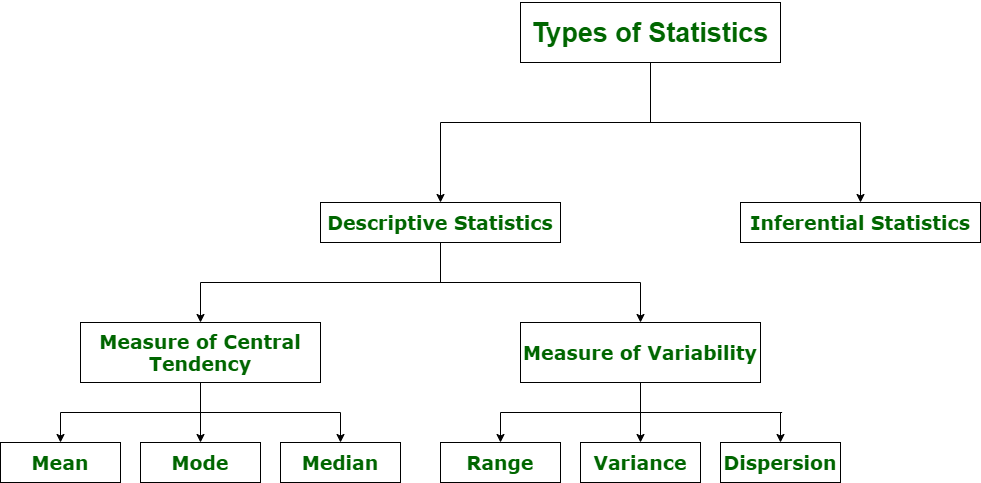
Mean, Median, and Mode

• Use Cases: The mean is often used when dealing with numerical data. It is sensitive to extreme values (outliers), so it may not be the best representation of central tendency when outliers are present.
• Example: When calculating the average test score in a class.

1. Median:

   • Use Cases: The median is robust to extreme values, making it a better choice when dealing with skewed distributions or datasets with outliers. It is especially useful when the data is not normally distributed.
   • Example: When determining the median income in a neighborhood.

2. Mode:

   • Use Cases: The mode is suitable for categorical data or discrete values. It represents the most frequently occurring value in a dataset.
   • Example: When identifying the most common blood type in a population.

Summary:

• Use the mean when dealing with numerical data and the distribution is roughly symmetric.
• Use the median when the data is skewed or has outliers, as it is less affected by extreme values.
• Use the mode when dealing with categorical or discrete data to identify the most common category or value.

It’s also important to note that in some cases, using multiple measures of central tendency can provide a more comprehensive understanding of the data. For example, reporting both the mean and median can give a sense of the data’s typical value while also indicating whether extreme values are influencing the mean.

mean = sum(x) / n

median = (x[n // 2] + x[(n - 1) // 2]) / 2 if n % 2 == 0 else x[n // 2]

count_dict = {}
for num in x:
    count_dict[num] = count_dict.get(num, 0) + 1

mode = [key for key, value in count_dict.items() if value == max(count_dict.values())][0]

Variance and Standard Deviation

Variance - Think of it as an average of how far each data point is from the mean, but squared (meaning the distance is magnified).Useful for understanding the spread of data, but the squared units can be hard to interpret directly.

Standard Deviation: This makes the units the same as the original data, which is easier to understand. Represents the typical distance a data point falls from the mean. A higher standard deviation indicates a larger spread of data points.

Difference between Variance & Standard Deviation¶

Variance is a method to find or obtain the measure between the variables that how are they different from one another, whereas standard deviation shows us how the data set or the variables differ from the mean or the average value from the data set.

Variance helps to find the distribution of data in a population from a mean, and standard deviation also helps to know the distribution of data in population, but standard deviation gives more clarity about the deviation of data from a mean.

mean = sum(x) / n

variance = sum((num - mean) ** 2 for num in x) / n

std_dev = variance ** 0.5

Why are they important?

They help you interpret the average (mean) of your data. A high mean with a high standard deviation tells you the data is spread out, while a high mean with a low standard deviation suggests the data points are clustered around the mean. They are used in various statistical tests to compare datasets, assess risk (e.g., financial markets), and build models based on the data’s distribution.

Weighted Mean

def weightedMean(X, W):
    # Write your code here
    wm = sum([X[i]*W[i] for i in range(len(X))])/sum(W)
    print("%.1f" % wm)

Quartiles

def median(arr):
    n = len(arr)
    return (arr[n // 2] + arr[(n - 1) // 2]) / 2 if n % 2 == 0 else arr[n // 2]

def quartiles(arr):
    arr.sort()
    n = len(arr)
    q2 = median(arr)
    q1 = median(arr[:n // 2])
    q3 = median(arr[(n + 1) // 2:])
    return q1, q2, q3

Interquartile Range

def interquartileRange(values, freqs):
    # Print your answer to 1 decimal place within this function
    x = [values[i] for i in range(len(values)) for _ in range(freqs[i])]
    q1, q2, q3 = quartiles(x)
    return q3 - q1

Kurtosis and skewness

Kurtosis and skewness are measures of the shape of a distribution.

1. Skewness:

   • Skewness measures the symmetry of a distribution.
   • A skewness value of 0 indicates a symmetrical distribution.
   • Positive skewness (greater than 0) indicates a distribution with a longer right tail, meaning it has more values on the left side of the distribution mean.
   • Negative skewness (less than 0) indicates a distribution with a longer left tail, meaning it has more values on the right side of the distribution mean.

2. Kurtosis:

   • Kurtosis measures the tail heaviness of a distribution.
   • A kurtosis value of 3 (excess kurtosis) is considered normal and indicates a distribution with tails similar to a normal distribution.
   • Excess kurtosis greater than 3 indicates heavier tails, which means more values in the tails compared to a normal distribution.
   • Excess kurtosis less than 3 indicates lighter tails, meaning fewer values in the tails compared to a normal distribution.

Interpreting the values:

• For skewness, a value closer to 0 indicates less skew. Positive or negative values indicate the direction of the skew.
• For kurtosis, a value of 3 indicates a normal distribution. Values above 3 indicate heavier tails, and values below 3 indicate lighter tails compared to a normal distribution.

It’s important to note that interpretation may vary depending on the context and the specific distribution of your data.

Shape of Data

i) Symmetric In the symmetric shape of the graph, the data is distributed the same on both sides. In symmetric data, the mean and median are located close together. The curve formed by this symmetric graph is called a normal curve.

ii) Skewness Skewness is the measure of the asymmetry of the distribution of data. The data is not symmetrical (i.e) it is skewed towards one side.

–> Skewness is classified into two types.

• Positive Skew

• Negative Skew

  1.Positively skewed:

In a Positively skewed distribution, the data values are clustered around the left side of the distribution and the right side is longer. The mean and median will be greater than the mode in the positive skew.

2.Negatively skewed

In a Negatively skewed distribution, the data values are clustered around the right side of the distribution and the left side is longer. The mean and median will be less than the mode.

iii) Kurtosis

Kurtosis is the measure of describing the distribution of data.

This data is distributed in different ways. They are:

• Platykurtic
• Mesokurtic

• Leptokurtic

  1.Platykurtic: The platykurtic shows a distribution with flat tails. Here the data is distributed faltly . The flat tails indicated the small outliers in the distribution.

  2.Mesokurtic: In Mesokurtic, the data is widely distributed. It is normally distributed and it also matches normal distribution.

  3.Leptokurtic: In leptokurtic, the data is very closely distributed. The height of the peak is greater than width of the peak.

Describing probability distributions and probability distributions with multiple variables

Sampling and Point estimation

Inferential Statistics¶ Back to Table of Contents

Inferential Statistics - offers methods to study experiments done on small samples of data and chalk out the inferences to the entire population (entire domain).

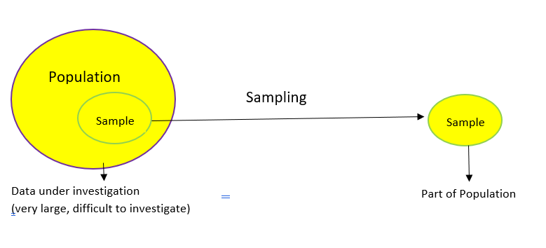
2.1 Population Vs Samples: In statistics, the population is a set of all elements or items that you’re interested in. Populations are often vast, which makes them inappropriate for collecting and analyzing data. That’s why statisticians usually try to make some conclusions about a population by choosing and examining a representative subset of that population.

This subset of a population is called a sample. Ideally, the sample should preserve the essential statistical features of the population to a satisfactory extent. That way, you’ll be able to use the sample to glean conclusions about the population.

Data Sampling:

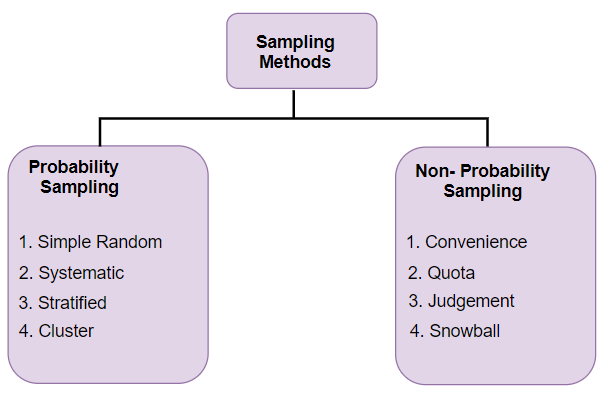
Data sampling is a statistical analysis technique used to select, manipulate and analyze a representative subset of data points to identify patterns and trends in the larger data set being examined. Different types of sampling technique:

Probability Sampling: In probability sampling, every element of the population has an equal chance of being selected. Probability sampling gives us the best chance to create a sample that is truly representative of the population Non-Probability Sampling: In non-probability sampling, all elements do not have an equal chance of being selected. Consequently, there is a significant risk of ending up with a non-representative sample which does not produce generalizable results

Population and Sampling

Sampling and Estimation: Sampling is a technique used to gather data from a smaller group to make inferences about a larger population. We can use this data to estimate certain characteristics of the population, such as the average or proportion.

population and sample.

• A population refers to the entire group of individuals or items that we want to study.
• A sample is a smaller subset of the population that we actually observe or measure.
• In machine learning and data science, we often use samples to train models and make predictions because we can’t look at the entire universe of data.
• When selecting a sample, it’s important to ensure that it is random and independent of previous samples.
• The sample should also be identically distributed, meaning that the rule used to pick the first sample should be the same for subsequent samples.
• In machine learning, every dataset we work with is actually a sample and not the population.
• It’s important to have a representative dataset that accurately reflects the distribution of the population.

Sample mean

• The content on this page discusses the concept of estimating population parameters using sample data.
• It uses the example of estimating the average height of the population in a fictional place called Statistopia.
• by taking a small sample from the population and calculating the average of the sample, we can estimate the average height of the entire population.
• It also highlights the importance of random sampling and how it affects the accuracy of the estimate.
• a larger sample size generally leads to a better estimate of the population mean.

sample proportion

• The population proportion (p) is the number of items with a given characteristic divided by the population size (n).
• The sample proportion (p hat) is an estimate of the population proportion, calculated by dividing the number of items with a given characteristic in a sample by the sample size.
• In the example given, the population proportion of people owning a bicycle is 40% (4 out of 10 people), while the sample proportion is 33.3% (2 out of 6 people).
• The sample proportion is used as an estimate of the population proportion when the population size is not known.

estimating population variance with a sample:

• Variance measures how much the values in a dataset deviate from the mean.
• The population variance is calculated using the formula Sigma squared, which is the average over the population size of x minus the population mean Mu squared.
• To estimate the population variance with a sample, you need to divide by the sample size minus one (n-1) instead of just the sample size (n).
• The formula for sample variance is the summation of (x minus the mean of the sample) squared divided by n-1.
• By taking multiple samples and calculating their variances, you can estimate the population variance.
• The estimated variance is obtained by averaging the variances of all the samples.

The formula for estimating the population variance with a sample is:

s^2 = Σ(x - x̄)^2 / (n - 1)

Where:

• s^2 represents the estimated population variance
• Σ denotes the summation symbol
• (x - x̄) represents the difference between each value in the sample and the sample mean
• n is the sample size

Law of Large Numbers:

The Law of Large Numbers states that as the sample size increases, the average of the sample will tend to get closer to the average of the entire population.

Conditions for the Law of Large Numbers to hold:

1. The samples must be drawn randomly from the population.
2. The sample size must be sufficiently large. The larger the sample size, the more accurate the sample mean is likely to be.
3. The individual observations in the sample must be independent of each other.

Central Limit Theorem - Discrete Random Variable:

• The Central Limit Theorem is a fundamental concept in statistics.
• It states that when you take multiple samples from any distribution and calculate their averages, the distribution of those averages will tend to follow a normal distribution.
• The example given is flipping a coin multiple times and counting the number of heads. As the number of coin flips increases, the distribution of the number of heads approaches a normal distribution.
• The mean of the distribution is equal to the number of coin flips multiplied by the probability of heads.
• The standard deviation of the distribution is equal to the square root of the number of coin flips multiplied by the probability of heads multiplied by the probability of tails.

Central Limit Theorem - Continuous Random Variable :

• The central limit theorem states that as the number of samples (n) increases, the distribution of the average of those samples approaches a standard normal distribution.
• The mean of the average (Yn) is the same as the population mean, while the variance of Yn is the population variance divided by the number of variables being averaged.
• The distribution of Yn becomes more bell-shaped and symmetric as n increases.
• The central limit theorem is usually true for n around 30 or higher, but in some cases, even smaller samples can exhibit a normal distribution.
• Standardizing the average makes it easier to compare distributions for different values of n.
• The more variables you average, the smaller the variance becomes, indicating less spread and less deviation from the population mean.
• The central limit theorem holds true regardless of the distribution of the original population.

Point Estimation

One common method of estimation is called maximum likelihood estimation (MLE). It is widely used in machine learning. MLE helps us estimate the parameters of a probability distribution. For example, if we have data that follows a certain pattern, MLE can help us figure out the most likely values for the parameters of that pattern.

Another method we discuss is called maximum a posteriori estimation (MAP). It is a Bayesian version of estimation. MAP takes into account not only the data but also our prior beliefs or assumptions about the parameters. It helps us find the most likely values for the parameters while considering our prior knowledge.

In simple terms, these methods help us make educated guesses about unknown values based on the information we have. MLE focuses on finding the most likely values based on the data, while MAP considers both the data and our prior beliefs. These methods are commonly used in machine learning to make accurate predictions and prevent overfitting.

MLE: Bernoulli Example:

• The example discussed in the content is about flipping a coin multiple times and trying to determine which coin was used based on the results.
• The concept of maximum likelihood was introduced, which involves finding the coin that maximizes the probability of obtaining the observed results.
• The likelihood function is the probability of observing the data given a specific model or parameter value.
• Taking the logarithm of the likelihood function simplifies calculations and allows for easier maximization.
• The optimal value of the parameter (in this case, the probability of heads) can be found by taking the derivative of the log likelihood function and setting it equal to zero.
• For a general case with multiple coins and heads, the optimal probability is equal to the mean of the population.

Interactive Tool: Likelihood Functions

MLE: Linear Regression:

• Maximum likelihood is used in machine learning to find the model that most likely generated the given data.
• In the example of fitting a line to data points, the best fit line is the one that gives the highest probability.
• The lines generate points close to the line, similar to houses being built close to a road.
• The points are generated using a Gaussian distribution centered at the intersection of the line and the horizontal line.
• The likelihood of generating a point is calculated using the formula of the Gaussian distribution.
• The likelihood of generating all the points is the product of the individual likelihoods.
• Maximizing the likelihood is the same as minimizing the sum of squared distances, which is the goal of linear regression.
• Finding the line that most likely produces the points using maximum likelihood is equivalent to minimizing the least square error in linear regression.

Regularization:

• Regularization is a technique used to prevent overfitting in machine learning models.
• It involves adding a penalty term to the loss function to discourage complex models.
• The penalty term is typically based on the sum of the squares of the model’s coefficients.
• The L2 regularization, also known as ridge regression, is a common form of regularization.
• The regularization parameter controls the strength of the penalty term.
• By applying regularization, we aim to find a simpler model that still fits the data well.
• Regularization is closely related to probability and maximum likelihood estimation.

“Introduction to Probability and Probability Distributions”:

• Probability is a measure of the likelihood of an event occurring.
• Probability distributions describe the possible outcomes and their associated probabilities.
• In the example given, there were three scenarios: movies, board games, and a nap, each with different probabilities of creating popcorn on the floor.
• The goal is to determine which scenario is most likely based on the evidence of popcorn on the floor.
• The probability of popcorn given movies was higher than the probability of popcorn given a popcorn throwing contest.
• However, the probability of watching movies by itself was much higher than the probability of a popcorn throwing contest.
• To factor in both probabilities, we multiply them together to find the probability of both events happening simultaneously.
• The goal is to maximize the probability of both events occurring, not just the conditional probability.

Here are your notes in Markdown format, including the formulae in LaTeX:

Bayesian Inference and MAP

There are two approaches to statistical inference: Bayesian and Frequentist. The method of Maximum Likelihood falls into the Frequentist category. Let’s explore some differences between the two approaches:

Frequentist vs. Bayesian

Frequentist	Bayesian
Probabilities represent long term frequencies	Probabilities represent a degree of belief, or certainty
Parameters are fixed (but unknown) constants	Make probability statements about parameters, even if they are constants (beliefs)
Find the model that better explains the observed data	Update beliefs on the model based on the observed data
Statistical procedures have well-defined long run frequency properties	Make inferences about a parameter $ \theta $ by producing a probability distribution for $ \theta $

The main difference between Frequentists and Bayesians is in the interpretation of probabilities.

• Frequentists: Probabilities represent long term relative frequencies, which is the frequency of appearance of a certain event in infinite repetitions of the experiment. This implies that probabilities are objective properties of the real world and that the parameters of the distribution are fixed constants; you might not know their value but the value is fixed. Since probabilities represent long term frequencies, Frequentists interpret observed data as samples from an unknown distribution, so it is natural to estimate models in a way that they explain the sampled data as best as possible.

• Bayesians: Probabilities represent a degree of belief. This belief applies to models as well. When you are Bayesian, even though you know the parameters take on a fixed value, you are interested in your beliefs about those values. Here is where the concept of prior is introduced. A prior is your baseline belief, what you believe about the parameter before you get new evidence or data. The goal of Bayesians is to update this belief as you gather new data. Your result will be an updated probability distribution for the parameter you are trying to infer. Using this distribution, you can later obtain different point estimates.

Example

Imagine you have four coins, three of which are fair and one biased with a probability of heads of 0.8. You choose randomly one of the four coins, and you want to know if you chose the biased one. You flip the coin 10 times and get 7 heads. Which coin did you choose?

A Frequentist would say that you chose the biased one because it has a higher likelihood:

$ L(0.8; 7H3T) = 0.8^7 \cdot 0.2^3 = 0.0018 > L(0.5; 7H3T) = 0.5^7 \cdot 0.5^3 = 0.00098 $

What would a Bayesian say? Notice that the frequentist didn’t take into account the fact that the biased coin had a 1 in 4 chance of being picked at the beginning. A Bayesian will try to exploit that information, as it will be their initial belief: without having any other information (observations), the chances of picking the biased coin are 1/4. The goal of a Bayesian is to update this belief, or probability, based on the observations.

Bayes’ Theorem

Remember from Week 1 of this course that Bayes’ theorem states that given two events $ A $ and $ B $:

$ P(B \mid A) = \frac{P(A \mid B) \cdot P(B)}{P(A)} $

But how can you use this to update the beliefs?

Notice that if the event $ B $ represents the event that the parameter takes a particular value, and the event $ A $ represents your observations (7 heads and 3 tails), then $ P(B) $ is your prior belief of how likely it is that you chose the biased coin before observing the data (0.25). $ P(A \mid B) $ is the probability of your data given the particular value of the parameter (probability of seeing 7 heads followed by 3 tails given that the probability of heads is 0.8). Finally, $ P(B \mid A) $ is the updated belief, which is called the posterior. Note that $ P(A) $ is simply a normalizing constant so that the posterior is well defined.

$ P(\text{Biased coin} \mid 7H3T) = \frac{P(7H3T \mid \text{Biased coin}) \cdot P(\text{Biased coin})}{P(7H3T)} = \frac{0.8^7 \cdot 0.2^3 \cdot 0.25}{0.8^7 \cdot 0.2^3 \cdot 0.25 + 0.5^7 \cdot 0.5^3 \cdot 0.75} = 0.364 $

Look how you went from a 0.25 confidence of choosing the biased coin to 0.364. Note that while your beliefs of having chosen the biased coin have increased, this still isn’t the most likely explanation. This is because you are taking into account the fact that originally your chances of choosing the biased coin were much smaller than choosing a fair one.

Relationship between MAP, MLE and Regularization

Certainly! Maximum likelihood estimation (MLE) and regularization are two important concepts in machine learning.

Maximum likelihood estimation is a method used to estimate the parameters of a statistical model based on observed data. It involves finding the values of the model’s parameters that maximize the likelihood of the observed data. In other words, MLE helps us find the most likely values for the parameters that would have generated the observed data.

On the other hand, regularization is a technique used to prevent overfitting in machine learning models. Overfitting occurs when a model becomes too complex and starts to fit the noise in the training data rather than the underlying patterns. Regularization helps to control the complexity of the model by adding a penalty term to the loss function, discouraging the model from assigning too much importance to any one feature or parameter.

Now, how do MLE and regularization relate to each other? In machine learning, when we perform regression with regularization, we aim to find the best model that fits the data while also considering the complexity of the model. Regularization helps us strike a balance between fitting the data well and avoiding overfitting.

When we add regularization to the loss function in regression, we are essentially adding a penalty term that discourages large parameter values. This penalty term helps to simplify the model and prevent it from becoming too complex. By doing so, we are implicitly incorporating a prior belief about the likelihood of different models. Simpler models are more likely to occur, while more complex models are less likely.

By combining the maximum likelihood estimation and regularization, we can find the best model that fits the data while also considering the complexity of the model. The regularization term helps us control the trade-off between fitting the data and keeping the model simple.

The relationship between Maximum Likelihood Estimation (MLE), Maximum A Posteriori (MAP) estimation, and regularization is as follows:

1. Maximum Likelihood Estimation (MLE):

   • MLE is a method used to estimate the parameters of a statistical model based on observed data.
   • It involves finding the values of the model’s parameters that maximize the likelihood of the observed data.
   • MLE assumes that the observed data is generated from a specific model, and it seeks to find the parameter values that make the observed data most likely.

2. Maximum A Posteriori (MAP) estimation:

   • MAP estimation is similar to MLE but incorporates prior knowledge or beliefs about the parameters of the model.
   • In addition to maximizing the likelihood of the observed data, MAP estimation also takes into account the prior probability distribution of the parameters.
   • The prior distribution represents our prior beliefs about the likely values of the parameters before observing any data.
   • By combining the likelihood and the prior, MAP estimation provides a way to find the parameter values that maximize the posterior probability of the parameters given the observed data.

3. Regularization:

   • Regularization is a technique used to prevent overfitting in machine learning models.
   • Overfitting occurs when a model becomes too complex and starts to fit the noise in the training data rather than the underlying patterns.
   • Regularization helps to control the complexity of the model by adding a penalty term to the loss function.
   • The penalty term discourages large parameter values, effectively simplifying the model and reducing overfitting.

The relationship between MLE, MAP estimation, and regularization can be understood as follows:

• MLE seeks to find the parameter values that maximize the likelihood of the observed data, assuming no prior knowledge or beliefs about the parameters.
• MAP estimation incorporates prior knowledge or beliefs about the parameters by combining the likelihood and the prior distribution.
• Regularization, when applied to MLE or MAP estimation, adds a penalty term to the loss function, encouraging the model to have smaller parameter values and reducing overfitting.

In summary, MLE and MAP estimation are methods for estimating model parameters, with MAP estimation incorporating prior knowledge. Regularization is a technique used to control model complexity and prevent overfitting, which can be applied to both MLE and MAP estimation.

Confidence Intervals and Hypothesis testing

Confidence Intervals and Hypothesis Testing: Confidence intervals help us estimate a range of values within which a population parameter is likely to fall. Hypothesis testing is a way to make decisions based on data, where we compare a hypothesis to the observed data to see if there is enough evidence to support or reject the hypothesis.

Z Distribution and Margin of Error:

Z Distribution:

• Confidence intervals are used to estimate an unknown population parameter with a certain degree of certainty.
• Instead of estimating a single point, a confidence interval provides a range of values within which the true parameter is likely to fall.
• The confidence level is determined by the significance level (alpha) and represents the frequency with which the sample means lie within the interval.
• A common value for alpha is 0.5, which corresponds to a confidence level of 95%.
• The lower and upper limits of the confidence interval are determined by the standard deviation and the confidence level chosen.
• The margin of error represents the standard deviation intervals defined by the confidence level and is added to the sample mean to obtain the confidence interval.
• The sample size affects the width of the confidence interval. As the sample size increases, the interval becomes narrower, providing a more precise estimate.
• The confidence level also affects the width of the confidence interval. A higher confidence level requires a wider interval to capture more area.
• The central limit theorem states that the sampling distribution of the sample means follows a normal distribution, with the mean equal to the population mean and the standard deviation equal to the population standard deviation divided by the square root of the sample size.

Margin of Error:

• Confidence intervals are used to estimate the range in which the population mean lies based on a sample mean.
• The confidence interval is calculated by adding and subtracting the margin of error from the sample mean.
• The margin of error is determined by multiplying the standard error (standard deviation divided by the square root of the sample size) with the critical value.
• The critical value is based on the desired confidence level, such as 95%, and is typically represented by the z-value.
• The z-value for a 95% confidence level is 1.96.
• The confidence interval captures the population mean with a certain level of confidence, such as 95% of the time.

The margin of error (MoE) is a measure of the uncertainty or potential error in the results of a survey or experiment. It represents the range within which the true value of the population parameter is expected to fall, given a certain level of confidence. The margin of error is typically associated with a confidence interval and can be calculated using the following steps:

Steps to Calculate Margin of Error

1. Determine the confidence level: Common confidence levels are 90%, 95%, and 99%. The confidence level indicates the probability that the margin of error contains the true population parameter.

2. Find the critical value (z or t): The critical value corresponds to the chosen confidence level. For large sample sizes (n > 30), you can use the z-distribution (normal distribution). For smaller sample sizes, you should use the t-distribution. Common z-scores for typical confidence levels are:

   • 90% confidence level: z ≈ 1.645
   • 95% confidence level: z ≈ 1.96
   • 99% confidence level: z ≈ 2.576

3. Calculate the standard error (SE):

   • For a population proportion $ p $: $ \text{SE} = \sqrt{\frac{p(1 - p)}{n}} $
   • For a population mean $ \mu $ (when the population standard deviation $ \sigma $ is known): $ \text{SE} = \frac{\sigma}{\sqrt{n}} $
   • For a population mean $ \mu $ (when the population standard deviation $ \sigma $ is unknown): $ \text{SE} = \frac{s}{\sqrt{n}} $ where $ s $ is the sample standard deviation.

4. Calculate the margin of error (MoE): $ \text{MoE} = z \times \text{SE} $ or for smaller samples: $ \text{MoE} = t \times \text{SE} $

Example Calculation

Suppose we have a sample proportion $ p $ of 0.5 (50%) from a survey of 1000 people, and we want to calculate the margin of error for a 95% confidence level.

1. Confidence level: 95%
2. Critical value: For a 95% confidence level, $ z \approx 1.96 $
3. Standard error: $ \text{SE} = \sqrt{\frac{p(1 - p)}{n}} = \sqrt{\frac{0.5(1 - 0.5)}{1000}} = \sqrt{\frac{0.25}{1000}} = \sqrt{0.00025} = 0.0158 $
4. Margin of error: $ \text{MoE} = z \times \text{SE} = 1.96 \times 0.0158 = 0.031 $

So, the margin of error is 0.031, or 3.1%. This means that the true population proportion is likely within 3.1% of the sample proportion, given a 95% confidence level.

Summary

The margin of error gives us an understanding of the precision of our estimate and allows us to construct confidence intervals to make inferences about the population parameter. The steps involve determining the confidence level, finding the critical value, calculating the standard error, and then computing the margin of error.

confidence intervals:

1. Confidence Interval:

• A confidence interval is a range of values that provides an estimate of an unknown population parameter.
• It is calculated based on a sample from the population and provides a measure of how confident we can be in our estimate.

1. Formula for Confidence Interval (for population mean):

• Confidence Interval = Sample Mean ± Margin of Error
• Margin of Error = Critical Value * Standard Error

1. Steps to Calculate a Confidence Interval:

• Step 1: Take a random sample from the population.
• Step 2: Calculate the sample mean (x̄) and sample standard deviation (s).
• Step 3: Choose a desired confidence level (e.g., 95%, 99%).
• Step 4: Find the critical value (z-value or t-value) corresponding to the chosen confidence level.
• Step 5: Calculate the standard error (SE) using the formula: SE = s / √(n), where n is the sample size.
• Step 6: Calculate the margin of error using the formula: Margin of Error = Critical Value * Standard Error.
• Step 7: Construct the confidence interval by adding and subtracting the margin of error from the sample mean.

1. Assumptions for Confidence Intervals:

• The sample used is random.
• The sample size is larger than 30, or the population is approximately normal.

Remember, these formulas and steps are specific to confidence intervals for population means. Different formulas and approaches may be used for confidence intervals for proportions or other population parameters.

Example confidence intervals and margin of error:

• Confidence intervals are used to estimate the range within which a population parameter, such as the mean, is likely to fall.

• The formula for calculating the margin of error is:

  Margin of Error = z * (standard deviation / square root of sample size)

  • z represents the critical value, which depends on the desired confidence level. For example, for a 95% confidence level, the critical value is typically 1.96.
  • The standard deviation (sigma) is a measure of the variability in the population.
  • The sample size (n) is the number of observations in the sample.

Here’s an example calculation using the formula:

• Let’s say we want to estimate the average height of adults in a population.
• We take a random sample of 49 adults and find that the sample mean height is 1 meter 70 centimeters.
• The population standard deviation is 25 centimeters.
• For a 95% confidence level, the critical value (z) is 1.96.

• Using the formula, the margin of error is calculated as:

  1.96 * (25 / sqrt(49)) = 7 centimeters.

• Therefore, the 95% confidence interval for the average height of adults in the population is 163 centimeters to 177 centimeters.

calculating sample size for a desired margin of error:

• The formula for calculating the sample size is: n ≥ (z * σ / MOE)^2, where:

  • n is the sample size
  • z is the z-score corresponding to the desired confidence level
  • σ is the standard deviation of the population
  • MOE is the desired margin of error

• To calculate the sample size, follow these steps:

  1. Determine the desired confidence level (e.g., 95% confidence level corresponds to a z-score of 1.96).
  2. Determine the standard deviation of the population (σ).
  3. Determine the desired margin of error (MOE).
  4. Substitute the values into the formula: n ≥ (z * σ / MOE)^2.
  5. Round up the result to the nearest whole number, as the sample size must be an integer.

• The formula helps determine the minimum sample size needed to achieve a desired margin of error. A larger sample size generally leads to a smaller margin of error and a more precise estimate of the population mean.

example calculating sample size for a desired margin of error:

Let’s say you are conducting a survey to estimate the average salary of engineers in your industry. You want to have a 95% confidence level and a margin of error of $500.

• Step 1: Determine the desired confidence level. In this case, it is 95%, which corresponds to a z-score of 1.96.

• Step 2: Determine the standard deviation of the population. Let’s assume that the standard deviation of salaries in your industry is $10,000 (σ = $10,000).

• Step 3: Determine the desired margin of error. In this case, it is $500 (MOE = $500).

• Step 4: Substitute the values into the formula: n ≥ (z * σ / MOE)^2.

  • n ≥ (1.96 * $10,000 / $500)^2
  • n ≥ (19.6)^2
  • n ≥ 384.16

• Step 5: Round up the result to the nearest whole number. In this case, the minimum sample size needed is 385.

Therefore, you would need to survey at least 385 engineers in order to estimate the average salary with a 95% confidence level and a margin of error of $500.

Difference Between Confidence and Probability:

• It explains the difference between saying that a confidence interval contains the true population parameter 95% of the time and saying that there is a 95% probability that the population parameter falls within the confidence interval.
• The population parameter, Mu, is fixed and unknown, while the sample mean has a probability distribution.
• The confidence interval is tied to the sample mean and changes depending on the value of the sample mean.
• Saying that you’re 95% confident has to do with the success rate of constructing the confidence interval, not the probability that a specific interval contains the population mean.

1. Population Parameter Mu:

   • Mu represents a characteristic or value of interest in the entire population.
   • It is fixed and unknown, meaning that it does not change but we don’t know its exact value.
   • Mu does not have a probability distribution because it is not random, it is just unknown.
   • It is always the same value for a given population.

2. Sample Mean:

   • The sample mean is a statistic that estimates the population parameter Mu.
   • It is calculated by taking the average of a sample from the population.
   • The sample mean has a probability distribution called the sampling distribution of the sample means.
   • The value of the sample mean can vary depending on the specific sample taken.

In summary, Mu is the fixed but unknown value of interest in the entire population, while the sample mean is a statistic that estimates Mu based on a sample. Mu does not have a probability distribution, but the sample mean does.

Student t-distribution:

• When we don’t know the standard deviation of the population, we use the sample standard deviation (s) instead.
• The sampling distribution with the sample standard deviation is called the Student t-distribution.
• The Student t-distribution is similar to the normal distribution but has fatter tails.

• To calculate the confidence interval when the standard deviation is unknown, we use the formula:

  Confidence Interval = x̄ ± t * (s / √n)

  • x̄ represents the sample mean.
  • t is the critical value from the Student t-distribution, which depends on the desired confidence level and the degrees of freedom.
  • s is the sample standard deviation.
  • n is the sample size.
• The degrees of freedom for the t-distribution are given by the number of samples minus 1.
• The larger the degrees of freedom, the closer the t-distribution resembles the normal distribution.

Why Use t and z Distributions?

The choice between the t-distribution and the z-distribution depends on the sample size and whether the population standard deviation is known:

1. z-Distribution:

   • Used when the sample size is large (typically $ n > 30 $).
   • The population standard deviation ($ \sigma $) is known.
   • The z-distribution is derived from the normal distribution and provides critical values for constructing confidence intervals.

2. t-Distribution:

   • Used when the sample size is small (typically $ n \leq 30 $).
   • The population standard deviation ($ \sigma $) is unknown and is estimated using the sample standard deviation ($ s $).
   • The t-distribution accounts for the extra uncertainty introduced by estimating the population standard deviation. It has heavier tails than the z-distribution, providing wider confidence intervals for small samples.

Real-World Example: Margin of Error Calculation

Let’s say we conducted a survey to estimate the average amount of time people spend on social media per day. We surveyed 25 people, and the sample mean ($ \bar{x} $) is 2 hours with a sample standard deviation ($ s $) of 0.5 hours. We want to calculate the margin of error for a 95% confidence interval.

1. Confidence Level: 95%
2. Sample Size: $ n = 25 $
3. Sample Mean: $ \bar{x} = 2 $ hours
4. Sample Standard Deviation: $ s = 0.5 $ hours

Since the sample size is small ($ n \leq 30 $), we’ll use the t-distribution.

Degrees of Freedom (df): $ df = n - 1 = 25 - 1 = 24 $

Critical Value (t): For a 95% confidence level and 24 degrees of freedom, the critical value $ t $ can be found using a t-table or statistical software. Let’s use a typical value: $ t \approx 2.064 $

Standard Error (SE): $ SE = \frac{s}{\sqrt{n}} = \frac{0.5}{\sqrt{25}} = \frac{0.5}{5} = 0.1 $

Margin of Error (MoE): $ \text{MoE} = t \times SE = 2.064 \times 0.1 = 0.2064 $

So, the margin of error is 0.2064 hours.

Interpretation

The average amount of time people spend on social media per day is estimated to be 2 hours, with a margin of error of 0.2064 hours, at a 95% confidence level. This means we can be 95% confident that the true average time spent on social media per day is between $ 2 - 0.2064 = 1.7936 $ hours and $ 2 + 0.2064 = 2.2064 $ hours.

Confidence Intervals for Proportion:

1. Confidence interval for proportions formula:

   • The confidence interval for proportions is given by p̂ ± margin of error.
   • p̂ represents the sample proportion.

2. Margin of error formula:

   • The margin of error is calculated using the formula: critical value * √(p̂ * (1 - p̂) / n).
   • The critical value depends on the desired confidence level.
   • p̂ represents the sample proportion.
   • n represents the sample size.

3. Standard deviation of a sampling distribution of proportions formula:

   • The standard deviation of a sampling distribution of proportions is given by √(p̂ * (1 - p̂) / n).
   • p̂ represents the sample proportion.
   • n represents the sample size.

To summarize:

• The confidence interval for proportions is given by p̂ ± margin of error.
• The margin of error is calculated using the formula: critical value * √(p̂ * (1 - p̂) / n).
• The standard deviation of a sampling distribution of proportions is given by √(p̂ * (1 - p̂) / n).

hypothesis testing

Defining Hypothesis:

• Hypothesis testing is a way to determine if a belief about a population is likely to be true or false.
• The null hypothesis (H0) is the base assumption, while the alternative hypothesis (H1) is the competing statement.
• The null and alternative hypotheses are mutually exclusive and have a true/false answer.
• The goal of hypothesis testing is to decide between the two hypotheses based on data and evidence.
• If there is enough evidence against the null hypothesis, it is rejected, and the alternative hypothesis is accepted as true.
• However, if the evidence is not sufficient, the null hypothesis is not rejected, but it doesn’t mean that the null hypothesis is true.
• A/B testing is an important application of hypothesis testing, often used in the field of data science and machine learning.
• A/B testing involves comparing two versions of something to determine which one performs better.

Type I and Type II errors:

1. Type I Error: This is when we mistakenly think something is true when it’s actually not. It’s like a false positive. For example, imagine you have an email spam filter. A type I error would be when the filter mistakenly marks a regular email as spam and sends it to the spam folder.

2. Type II Error: This is when we mistakenly think something is not true when it actually is. It’s like a false negative. Using the same example, a type II error would be when the spam filter fails to identify a spam email and lets it into your inbox.

In summary:

• Type I Error: Mistakenly thinking something is true when it’s not (false positive).
• Type II Error: Mistakenly thinking something is not true when it actually is (false negative).

The goal is to minimize both types of errors, but it’s important to understand that reducing one type of error may increase the other. So, it’s about finding a balance based on the significance level (alpha) and the specific context of the decision you’re making.

significance level (alpha)

The significance level (alpha) plays a crucial role in determining the balance between type I and type II errors. Here’s how it affects the balance:

1. Significance Level (alpha): The significance level represents the maximum probability of making a type I error (rejecting a null hypothesis when it is actually true). It is usually denoted by the Greek letter alpha. The significance level is a design criterion for hypothesis testing.

2. Balance between Type I and Type II Errors: As you decrease the significance level (alpha), you are reducing the probability of making a type I error. This means you become more cautious about rejecting the null hypothesis and making false positive conclusions. However, reducing the probability of a type I error too much can increase the probability of making a type II error (failing to reject the null hypothesis when it is actually false).

3. Trade-off: There is a trade-off between type I and type II errors. If you set a very low significance level (alpha), you are being more stringent in accepting evidence against the null hypothesis. This reduces the chances of false positives (type I errors) but increases the chances of false negatives (type II errors). On the other hand, if you set a higher significance level, you become more lenient in accepting evidence against the null hypothesis, which increases the chances of false positives but decreases the chances of false negatives.

In summary, the significance level (alpha) determines the threshold for rejecting the null hypothesis. By adjusting the significance level, you can control the balance between type I and type II errors. It’s important to strike a balance that aligns with the specific context and consequences of the decision you’re making.

right-tailed, left-tailed, and two-tailed hypothesis tests:

1. Right-tailed test:

   • In a right-tailed test, the alternative hypothesis (H1) extends to the right of the null hypothesis (H0).
   • It is used when you want to determine if a population parameter is greater than a certain value.
   • The critical region for rejection is in the right tail of the distribution.
   • Type I error occurs when you reject the null hypothesis when it is actually true.
   • Type II error occurs when you fail to reject the null hypothesis when it is actually false.

2. Left-tailed test:

   • In a left-tailed test, the alternative hypothesis (H1) extends to the left of the null hypothesis (H0).
   • It is used when you want to determine if a population parameter is less than a certain value.
   • The critical region for rejection is in the left tail of the distribution.
   • Type I error occurs when you reject the null hypothesis when it is actually true.
   • Type II error occurs when you fail to reject the null hypothesis when it is actually false.

3. Two-tailed test:

   • In a two-tailed test, the alternative hypothesis (H1) states that the population parameter is different from the null hypothesis (H0).
   • It is used when you want to determine if a population parameter is not equal to a certain value.
   • The critical region for rejection is split between the two tails of the distribution.
   • Type I error occurs when you reject the null hypothesis when it is actually true.
   • Type II error occurs when you fail to reject the null hypothesis when it is actually false.

In summary, the choice between a right-tailed, left-tailed, or two-tailed test depends on the specific research question and the directionality of the hypothesis being tested.

p-Value:

• The intuition is that if your sample mean falls too far away from the null hypothesis, then you reject H_0.
• The sample mean has a Gaussian distribution with parameters Mu=66.7 and standard deviation 3 divided by square root 10, assuming H_0 is true.
• The p-value is a probability, assuming H_0 is true, that the test statistic takes on a value as extreme as or more extreme than the observed value.
• The p-value is a good metric to create a decision rule for the test. If the p-value is less than Alpha, you reject H_0 and accept H_1 is true. If the p-value is bigger than Alpha, you don’t reject H_0.
• For a right-tailed test, the p-value is the probability of the test statistic being greater than the observed value under the assumption that H_0 is true.
• For a two-tail test, the p-value is the probability of all points that are distance from Mu_0 greater than the observed value in both directions.
• For a left-tailed test, the p-value is the probability that the test statistic is smaller than the observed value, assuming H_0 is true.
• The z-statistic is the standardized version of x-bar. If H_0 is true, then the z-statistic follows a standard normal distribution.

Critical Values:

• Critical values are used to make decisions in hypothesis testing.
• The critical value is the most extreme sample value that would still lead to rejecting the null hypothesis.
• It depends on the significance level (Alpha) chosen for the test.
• Different significance levels result in different critical values.
• Critical values can be used to create a decision rule for hypothesis testing.
• The decision rule is based on comparing the observed sample statistic to the critical value.
• Critical values can be determined in advance, before collecting any data.
• The P-value method and the critical value method should lead to the same conclusion.
• Critical values allow for the determination of type 2 error probabilities.

Here is the formula for finding the critical value for a right-tail test:

K_alpha = quantile(1 - Alpha)

For a left-tail test:

K_alpha = quantile(Alpha)

And for a two-tailed test:

K_alpha1 = quantile(1 - Alpha/2)
K_alpha2 = quantile(Alpha/2)

Power of a Test

understanding the chances of making errors when we analyze data. There are two types of errors we need to be aware of: Type I and Type II errors.

• Type I error happens when we reject a statement or hypothesis that is actually true. It’s like saying something is wrong when it’s actually right.
• Type II error happens when we fail to reject a statement or hypothesis that is actually false. It’s like saying something is right when it’s actually wrong.

To avoid these errors, we use statistical tests and make decisions based on certain rules. The probability of making a Type I error is called the significance level, and it’s something we choose before conducting the test. The probability of making a Type II error is called beta, and it depends on the true value of what we are testing.

We also have something called the power of the test, which is the probability of making the right decision and rejecting a false statement. It complements the Type II error probability. So, the power of the test is 1 minus the probability of making a Type II error.

The power of the test and the probability of a Type II error are closely related. In fact, they are complementary to each other.

• The power of the test is the probability of making the correct decision and rejecting a false statement or hypothesis. It tells us how likely we are to correctly identify something as true when it is indeed true.

• On the other hand, the probability of a Type II error is the probability of failing to reject a false statement or hypothesis. It tells us how likely we are to incorrectly accept something as true when it is actually false.

Mathematically, the power of the test can be calculated as 1 minus the probability of a Type II error. So, if the probability of a Type II error is denoted as beta, then the power of the test is 1 - beta.

t-distribution:

• The t-distribution is a probability distribution that is used when the population standard deviation is unknown.
• It is similar to the normal distribution, but with heavier tails.
• The t-distribution is characterized by its degrees of freedom (denoted as ν), which control the shape of the distribution.
• The formula for the t-statistic is: t = (x̄ - μ) / (s / √n), where x̄ is the sample mean, μ is the population mean, s is the sample standard deviation, and n is the sample size.
• The degrees of freedom for the t-distribution is equal to the sample size minus one (ν = n - 1).
• Hypothesis testing involves comparing the t-statistic to critical values from the t-distribution to determine if there is a significant difference between the sample mean and the population mean.
• The critical values are determined based on the desired level of significance (α) and the degrees of freedom.
• If the t-statistic falls within the critical region, we reject the null hypothesis and conclude that there is a significant difference.
• If the t-statistic falls outside the critical region, we fail to reject the null hypothesis and conclude that there is not enough evidence to support a significant difference.

Two-Tail Test with the t Statistic

In a two-tail test using the t statistic, the p-value is calculated as follows:

1. Calculate the observed t statistic from the sample data.
2. Determine the degrees of freedom (df) for the test.
3. Look up the critical value for the desired significance level and the degrees of freedom in the t-distribution table.
4. Calculate the p-value by finding the probability of the t statistic being greater than the observed t statistic (in absolute value) and multiply it by 2.

The formula for calculating the p-value for a two-tail test using the t statistic is:

p-value = 2 * (1 - CDF(t_observed, df))

Where:

• p-value is the probability value
• CDF is the cumulative distribution function of the t-distribution
• t_observed is the observed t statistic
• df is the degrees of freedom

Remember to use the absolute value of the observed t statistic when calculating the probability.

ML Application: A/B Testing

Sure! The content on this page is about A/B testing, which is a method used to compare two variations and make data-driven decisions. It explains how A/B testing is a broader methodology that includes various steps, and the t-Test is one statistical tool used in A/B testing. The page provides an example of A/B testing for a website’s buy now button placement and another example for testing different website designs. It also discusses the statistical calculations involved in A/B testing, such as hypothesis testing and calculating p-values. Overall, the content emphasizes the importance of using statistical tools like the t-Test to analyze data and make informed decisions in A/B testing.

A/B Testing

A/B testing is a method used to compare two variations and make data-driven decisions. It involves several steps:

1. Propose the variation: Identify the specific changes or variations you want to test.
2. Randomly split the sample: Divide your sample subjects into two groups, with each group exposed to a different variation.
3. Measure the outcomes: Collect data on the performance or behavior of each group.
4. Determine metrics: Define the metrics or measurements you will use to evaluate the variations, such as mean behavior, proportions, or dispersion.
5. Apply statistical tools: Use statistical tests to analyze the data and make a decision based on the results.

Two-Sample t-Test

In the example of A/B testing for a website’s buy now button placement, a two-sample t-Test is used to compare the mean purchase amounts for two strategies (A and B). The formulas involved are:

• Null hypothesis: $ H_0: \mu_A = \mu_B $ (the mean purchase amounts for both strategies are the same)
• Alternative hypothesis: $ H_1: \mu_B > \mu_A $ (the mean purchase amount for Strategy B is larger than Strategy A)

The test statistic for the two-sample t-Test is calculated as follows:

\[t = \frac{\overline{X}_A - \overline{X}_B}{\sqrt{\frac{s_A^2}{n_A} + \frac{s_B^2}{n_B}}}\]

Where:

• $ \overline{X}_A $: Sample mean purchase amount for Strategy A
• $ \overline{X}_B $: Sample mean purchase amount for Strategy B
• $ s_A $: Sample standard deviation for Strategy A
• $ s_B $: Sample standard deviation for Strategy B
• $ n_A $: Number of observations for Strategy A
• $ n_B $: Number of observations for Strategy B

The degrees of freedom for the t-distribution can be calculated using the formula:

\[df = \frac{\left(\frac{s_A^2}{n_A} + \frac{s_B^2}{n_B}\right)^2}{\frac{\left(\frac{s_A^2}{n_A}\right)^2}{n_A - 1} + \frac{\left(\frac{s_B^2}{n_B}\right)^2}{n_B - 1}}\]

Binomial Test

In another example of A/B testing for website design, a binomial test is used to compare the conversion rates of two designs (A and B). The formulas involved are:

• Null hypothesis: $ H_0: p_A = p_B $ (the conversion rates for both designs are the same)
• Alternative hypothesis: $ H_1: p_B > p_A $ (the conversion rate for Design B is higher than Design A)

The test statistic for the binomial test is calculated as follows:

\[z = \frac{\hat{p} - p_0}{\sqrt{\frac{p_0 (1 - p_0)}{n}}}\]

Where:

• $ X $: Number of conversions for a specific design
• $ n $: Total number of observations for that design
• $ \hat{p} $: Estimated conversion rate $ \left( \frac{X}{n} \right) $
• $ p_0 $: Hypothesized population proportion

The observed test statistic is compared to the critical value or p-value to make a decision.

ANOVA (Analysis of Variance)

Definition:

ANOVA is a statistical technique used to compare the means of two or more groups to determine if there are any statistically significant differences between them. It helps in understanding whether the variation in the data is due to the effect of the independent variable(s) or due to random chance.

Key Concepts:

1. Groups (Levels): Different categories or treatments being compared.
2. Dependent Variable: The outcome variable that is measured in the study.
3. Independent Variable: The factor or factors being manipulated to observe their effect on the dependent variable.
4. Between-Group Variance: Variation due to the differences between the groups.
5. Within-Group Variance: Variation due to differences within each group.

Types of ANOVA:

1. One-Way ANOVA: Compares the means of three or more unrelated groups based on one independent variable.
2. Two-Way ANOVA: Compares the means based on two independent variables and can also evaluate the interaction effect between them.
3. Repeated Measures ANOVA: Compares the means of the same group at different times or under different conditions.

Process:

1. Hypotheses Formulation:

   • Null Hypothesis ($H_0$): The means of the groups are equal.
   • Alternative Hypothesis ($H_1$): At least one group mean is different.

2. Calculating ANOVA:

   • Sum of Squares Between (SSB): Measures the variance between the groups.
   • Sum of Squares Within (SSW): Measures the variance within each group.
   • Total Sum of Squares (SST): The total variance in the data.

   $ SST = SSB + SSW $

   • Mean Square Between (MSB): Average between-group variance.

   $ MSB = \frac{SSB}{df_{between}} $

   • Mean Square Within (MSW): Average within-group variance.

   $ MSW = \frac{SSW}{df_{within}} $

   • F-Ratio: Ratio of between-group variance to within-group variance.

   $ F = \frac{MSB}{MSW} $

3. Decision Making:

   • Calculate the F-statistic using the F-distribution table based on the degrees of freedom.
   • Compare the calculated F-value with the critical F-value from the table at a chosen significance level (e.g., $\alpha = 0.05$).

   • Determine the p-value corresponding to the F-statistic.

   • If $ p \leq \alpha $, reject the null hypothesis ($H_0$).
   • If $ p > \alpha $, fail to reject the null hypothesis ($H_0$).

Assumptions:

1. Independence: Observations within each group must be independent.
2. Normality: The data within each group should be approximately normally distributed.
3. Homogeneity of Variances: The variance among the groups should be approximately equal (homoscedasticity).

Applications:

ANOVA is widely used in various fields such as:

• Psychology: To compare the effectiveness of different therapies.
• Agriculture: To evaluate the impact of different fertilizers on crop yield.
• Medicine: To compare the effects of different drugs on patient recovery rates.
• Business: To assess the impact of different marketing strategies on sales.

Example:

Consider a study to compare the test scores of students from three different teaching methods (A, B, C).

1. Formulate the hypotheses:

   • $H_0$: Mean scores of students in all three methods are equal.
   • $H_1$: At least one mean score is different.
2. Collect and organize the data.
3. Calculate SSB, SSW, MSB, MSW, and the F-ratio.
4. Determine the p-value and compare it with the significance level.
5. Draw conclusions based on the results.

Conclusion:

ANOVA is a powerful statistical tool for comparing means across multiple groups and determining if the differences are statistically significant. By following the process and ensuring assumptions are met, researchers can make informed decisions about the effects of different factors on a dependent variable.

Analysis in Machine Learning

Regression analysis

Types of Analysis in Machine Learning

1. Univariate Analysis

Definition: Univariate analysis involves analyzing a single variable. The purpose is to describe the data and find patterns that exist within it.

Identification:

• Look at the dataset and identify if you’re dealing with only one variable.
• Common methods include frequency distribution, central tendency measures (mean, median, mode), dispersion measures (range, variance, standard deviation), and visualizations (histograms, box plots).

Handling in ML:

• Preprocessing: Handle missing values, detect outliers, and apply transformations (e.g., log transformation).
• Feature Engineering: Create new features based on the univariate distribution (e.g., binning continuous variables).

2. Bivariate Analysis

Definition: Bivariate analysis involves the analysis of two variables to understand the relationship between them.

Identification:

• Look at the dataset and identify if you’re dealing with two variables.
• Common methods include scatter plots, correlation coefficients (Pearson, Spearman), cross-tabulations, and bivariate plots.

Handling in ML:

• Feature Engineering: Create interaction terms, ratio features, or difference features.
• Preprocessing: Normalize or standardize features if necessary.

3. Multivariate Analysis

Definition: Multivariate analysis involves the analysis of more than two variables to understand relationships and interactions among them.

Identification:

• Look at the dataset and identify if you’re dealing with multiple variables.
• Common methods include multiple regression analysis, principal component analysis (PCA), factor analysis, and cluster analysis.

Handling in ML:

• Dimensionality Reduction: Use techniques like PCA or t-SNE to reduce the number of features while retaining important information.
• Feature Selection: Use techniques like forward selection, backward elimination, or regularization methods (Lasso, Ridge) to select important features.
• Handling Multicollinearity: Detect multicollinearity using variance inflation factor (VIF) and address it by removing highly correlated variables or combining them.

4. Time Series Analysis

Definition: Time series analysis involves analyzing data points collected or recorded at specific time intervals to identify trends, seasonal patterns, and cycles.

Identification:

• Look for datasets with a time component (e.g., dates, timestamps).
• Common methods include autocorrelation plots, seasonal decomposition, and time series forecasting models (ARIMA, Exponential Smoothing).

Handling in ML:

• Preprocessing: Handle missing values, apply transformations (e.g., differencing), and create lag features.
• Feature Engineering: Create time-based features like day of the week, month, or quarter.
• Modeling: Use specialized time series models like ARIMA, Prophet, or LSTM for forecasting.

5. Spatial Analysis

Definition: Spatial analysis involves analyzing data that has a geographical or spatial component.

Identification:

• Look for datasets with spatial information (e.g., latitude, longitude).
• Common methods include spatial autocorrelation, kriging, and spatial regression.

Handling in ML:

• Preprocessing: Handle missing spatial data and apply spatial transformations.
• Feature Engineering: Create spatial features like distance to important locations, spatial clusters, or regional averages.
• Modeling: Use spatial models or incorporate spatial features into traditional models.

Summary

Steps to Identify the Type of Analysis:

1. Examine the dataset to identify the number of variables and their types.
2. Determine if there is a time component or spatial component.
3. Use appropriate visualization and statistical methods to explore the relationships.

Handling in ML:

• Preprocess the data accordingly.
• Use feature engineering to create meaningful features.
• Choose appropriate models and techniques based on the type of analysis.

Understanding the type of analysis and how to handle it in machine learning is crucial for building accurate and effective models. Always start with exploratory data analysis (EDA) to gain insights and guide your preprocessing and modeling steps.

Inadequate Reasoning in Statistical Analysis

1. Correlation vs. Causation

• Issue: Assuming causation based on correlation.
• Example: Single-sex schools show better results for girls, but multiple factors like socioeconomic status and selectivity may influence the outcome.

2. Misunderstanding Randomness

• Issue: Misinterpreting natural randomness, especially in sample size effects.
• Example: A smaller hospital with fewer daily births may show more variability in the proportion of boys born due to its smaller sample size.

3. Ecological Fallacy

• Issue: Attributing characteristics to individuals based on group characteristics.
• Example: Assuming everyone in a census area earns $50,000 p.a. when individual incomes within the group can vary widely.

4. Atomistic Fallacy

• Issue: Generalizing characteristics based on an unrepresentative sample.
• Example: Drawing conclusions about a population from a small or biased sample that may not accurately represent the whole.

5. Misinterpretation of Visualizations

• Issue: Incorrectly interpreting data presented visually.
• Example: Misleading interpretation of prostate cancer survival rates due to outdated data, differences in screening practices, and incorrect deduction of survival rates from raw diagnosis and mortality data.

6. Prosecutor’s Fallacy

• Issue: Assuming guilt based on the probability of evidence, without considering other possibilities.
• Example: Claiming a one-in-a-million chance of innocence based on rare evidence, without accounting for the overall population.

7. Overreliance on Past Events

• Issue: Assuming past random events influence future outcomes.
• Example: Believing that a coin is more likely to land heads after a series of tails, without considering each toss’s independent probability.

8. Lack of Consideration for Confounding Variables

• Issue: Neglecting third variables that could influence observed correlations.
• Example: Linking high fat consumption to breast cancer without considering other factors like genetics, lifestyle, or overall health.

9. Time Dependency in Data

• Issue: Drawing conclusions without considering changes over time.
• Example: Using outdated data on prostate cancer survival rates without accounting for improvements in treatment and healthcare practices.

10. Lack of Context in Data Interpretation

• Issue: Failing to consider contextual factors that impact conclusions.
• Example: Interpreting declining teenage pregnancy rates without accounting for cyclical patterns and selective reporting.

In statistical analysis, addressing these issues requires careful consideration of study design, awareness of potential biases, and a cautious approach to drawing causal relationships from observed correlations.

Correlation in Statistics

Correlation in statistics measures the relationship between paired datasets. It doesn’t imply causation but can suggest a potential causal relationship. For example, the correlation between global temperature rise and carbon dioxide emissions may indicate a relationship, but other factors might also contribute.

Independence and Correlation

If two variables show no correlation, they are likely independent. Detecting correlation prompts questioning of independence and examination of potential dependent relationships. The terms “independent variable” and “dependent variable” are used to explore how one variable may influence another.

Correlation Coefficient

The correlation coefficient quantifies the degree of correlation between variables. The most common is the Pearson correlation coefficient, ranging from -1 to +1:

• 0: No correlation
• +1: Perfect positive correlation
• -1: Perfect negative (inverse) correlation

Pearson Correlation Coefficient (r)

The Pearson correlation coefficient (r) measures the linear relationship between two variables, $ x $ and $ y $. It is calculated as the ratio of covariance to the product of standard deviations:

\[r_{xy} = \frac{\text{cov}(x, y)}{s_x \cdot s_y}\]

Where:

• $\text{cov}(x, y)$ is the covariance of $ x $ and $ y $
• $s_x$ and $s_y$ are the standard deviations of $ x $ and $ y $

When to Use:

• When you have two continuous variables and want to measure the strength and direction of their linear relationship.
• Example: Examining the relationship between hours studied and exam scores.

Significance:

• Use a significance test (like the t-test) to determine if the correlation coefficient is significantly different from zero.
• A p-value less than the chosen significance level (e.g., 0.05) indicates a significant correlation.

Calculation

1. Covariance: \(\text{cov}(x, y) = S_{xy} = \frac{\sum (x_i - \bar{x})(y_i - \bar{y})}{n-1}\)
2. Standard Deviations: \(s_x = \sqrt{\frac{\sum (x_i - \bar{x})^2}{n-1}}\)
3. Pearson Correlation Coefficient: \(r_{xy} = \frac{\sum (x_i - \bar{x})(y_i - \bar{y})}{\sqrt{\sum (x_i - \bar{x})^2 \sum (y_i - \bar{y})^2}}\)

def pearson_correlation_coefficient(x, y):
    n = len(x)
    mean_x = sum(x) / n
    mean_y = sum(y) / n
    covariance = sum((x[i] - mean_x) * (y[i] - mean_y) for i in range(n))
    std_dev_x = (sum((xi - mean_x) ** 2 for xi in x) / n) ** 0.5
    std_dev_y = (sum((yi - mean_y) ** 2 for yi in y) / n) ** 0.5
    correlation_coefficient = covariance / (n * std_dev_x * std_dev_y)
    return correlation_coefficient

Spearman’s Rank Correlation (ρ)

Spearman’s rank correlation measures the monotonic relationship between paired observations. It is calculated using the difference in ranks (d) of the observations:

\[\rho = 1 - \frac{6 \sum d_i^2}{n(n^2 - 1)}\]

Where:

• $ d_i = \text{rank}(x_i) - \text{rank}(y_i) $
• $ n $ is the number of observations

When to Use:

• When you have ordinal data or when the relationship between variables is not linear.
• Example: Ranking students based on their test scores and class participation.

Significance:

• Use a significance test (like the t-distribution with (n-2) degrees of freedom) to determine if the rank correlation is significantly different from zero.
• A p-value less than the chosen significance level (e.g., 0.05) indicates a significant correlation.

def spearman_rank_correlation(x, y):
    n = len(x)
    x_s = sorted(x)
    y_s = sorted(y)
    x_r = [x_s.index(ele) + 1 for ele in x]
    y_r = [y_s.index(ele) + 1 for ele in y]
    d_sqr = [(x_r[i] - y_r[i])**2 for i in range(n)]
    r = 1 - ((6 * sum(d_sqr)) / (n * (n**2 - 1)))
    return r

Kendall’s Rank Correlation (τB)

Kendall’s rank correlation measures the concordance or discordance between pairs of observations. It is calculated as:

\[\tau_B = \frac{N_c - N_d}{\frac{1}{2}n(n-1)}\]

Where:

• $ N_c $ is the number of concordant pairs
• $ N_d $ is the number of discordant pairs

When to Use:

• When you have small sample sizes or when you want a measure that handles ties well.
• Example: Analyzing the consistency of rankings given by two judges.

Significance:

• For larger sample sizes (n > 10), use the Normal distribution to assess significance.
• A p-value less than the chosen significance level (e.g., 0.05) indicates a significant correlation.

Scale Dependency

Scale dependency refers to the impact of scale, grouping, and arrangement on data analysis. It can reveal different patterns, like in the Yule-Simpson effect or Simpson’s Paradox, where grouped data can show different correlations compared to ungrouped data.

When to Use:

• When analyzing data with potential grouping or scaling effects.
• Example: Investigating if the correlation between education level and income varies by geographic region.

Confidence Intervals and Bootstrapping

Bootstrapping is a resampling technique used to estimate the distribution of a statistic. It involves generating multiple datasets by random sampling with replacement and computing correlation coefficients. Confidence intervals can be obtained from these bootstrapped distributions.

When to Use:

• When you need robust estimates of confidence intervals for correlation coefficients, especially with small sample sizes.
• Example: Estimating the confidence interval for the correlation between income and expenditure.

Correlation Matrix

In datasets with multiple variables, a correlation matrix shows pairwise correlation coefficients. Visualization tools like correlograms help in interpreting these relationships.

When to Use:

• When analyzing datasets with many variables to understand the pairwise relationships between them.
• Example: Creating a correlation matrix to study relationships among various financial indicators.

Partial Correlation

Partial correlation examines the relationship between two variables while controlling for a third variable. This helps isolate specific relationships by removing the influence of other variables.

When to Use:

• When you need to understand the direct relationship between two variables while controlling for the effect of other variables.
• Example: Studying the relationship between exercise and weight loss while controlling for diet.

Correlograms

Correlograms display the variation in correlation against an ordered variable, such as time or distance. They are useful for exploring data patterns over time or space.

When to Use:

• When analyzing time series or spatial data to understand how correlations change over time or distance.
• Example: Using a correlogram to study the autocorrelation of monthly sales data.

statistical concepts

1. Descriptive Statistics:

   • Definition: Descriptive statistics involve methods and measures that describe the data.
   • Key Components:
     • Measures of Central Tendency (Mean, Median, Mode).They help us understand where the “average” or “central” point lies amidst a collection of data points.
     • Measures of Variability (Range, Variance, Standard Deviation, Quartile Range).These provide valuable insights into the degree of variability or uniformity in the data.

2. Inferential Statistics:

   • Definition: Inferential statistics draw conclusions about a population from a sample, using techniques like hypothesis testing and regression analysis to determine the likelihood of observed patterns occurring by chance and to estimate population parameters.
   • Importance: Enables data scientists to make data-driven decisions and formulate hypotheses about broader contexts.

3. Probability Distributions:

   • Definition: Probability distributions provide a structured framework for characterizing the probabilities of various outcomes in random events.
   • Key Distributions: Normal, Binomial, Poisson.
   • Significance: Essential for statistical analysis, hypothesis testing, and predictive modeling.

4. Sampling Methods:

   • Importance: Ensures that the sample is representative of the population in inferential statistics.

   • Common Methods:

     • Simple Random Sampling: Each member of the population has an equal chance of being selected for the sample through random processes.

     • Stratified Sampling: Population is divided into subgroups (strata), and a random sample is taken from each stratum in proportion to its size.

     • Systematic Sampling: Selecting every “kth” element from a population list, using a systematic approach to create the sample.

     • Cluster Sampling: Population is divided into clusters, and a random sample of clusters is selected, with all members in selected clusters included.

     • Convenience Sampling: Selection of individuals/items based on convenience or availability, often leading to non-representative samples.

     • Purposive (Judgmental) Sampling: Researchers deliberately select specific individuals/items based on their expertise or judgment, potentially introducing bias.

     • Quota Sampling: The population is divided into subgroups, and individuals are purposively selected from each subgroup to meet predetermined quotas.

     • Snowball Sampling: Used in hard-to-reach populations, where participants refer researchers to others, leading to an expanding sample.

5. Regression Analysis:

   • Definition: Quantifies the relationship between a dependent variable and one or more independent variables.
   • Models: Linear Regression, Logistic Regression.
   • Applications: Used in various fields for predicting and understanding relationships.

6. Hypothesis Testing:

   • Definition: Assesses claims or hypotheses about a population using sample data.
   • Process: Formulate null and alternative hypotheses, use statistical tests to evaluate support for the alternative hypothesis.

7. Data Visualizations:

   • Definition: Represents complex data visually for easy comprehension.
   • Importance: Enables the identification of trends, patterns, and outliers, facilitating data analysis and decision-making.

8. ANOVA (Analysis of Variance):

   • Definition: Compares means of two or more groups to determine significant differences.
   • Process: Calculates a test statistic and p-value to assess whether observed differences are statistically significant.
   • Applications: Widely used in research to assess the impact of different factors on a dependent variable.

9. Time Series Analysis:

   • Definition: Focuses on studying data points collected over time to understand patterns and trends.
   • Techniques: Data visualization, smoothing, forecasting, and modeling.
   • Applications: Used in finance, economics, climate science, and stock market predictions.

10. Bayesian Statistics:

    • Definition: Bayesian statistics treats probability as a measure of uncertainty, updating beliefs based on prior information and new evidence.
    • Applications: Particularly useful for complex, uncertain, or small-sample data in fields like machine learning, Bayesian networks, and decision analysis.